
Event held online
Conference proceedings
ECB Forum on Central Banking, November 2020
1
Contents
Programme 3
Central banks in a shifting world: takeaways from the ECB’s online
Sintra Forum 5
By Philipp Hartmann and Glenn Schepens
Monetary policy in a pandemic emergency 20
By Christine Lagarde
De-globalisation? Global value chains in the post-COVID-19 age 28
By Pol Antràs
De-globalisation? The recent slowdown of global trade and prospects
for future rebalancing 81
By Susan Lund
Macro-financial implications of climate change and the carbon transition 90
By Frederick van der Ploeg
Discussion of "Macro-financial implications of climate change and the
carbon transition" by Frederick van der Ploeg 143
By Signe Krogstrup
The decline in r* and the ECB strategy 151
By Jordi Galí
Informal central bank communication 156
By Annette Vissing-Jorgensen
The decline in euro area inflation and the choice of policy strategy 169
By Volker Wieland
Monetary policy challenges from falling natural interest rates 186
By Klaus Adam
Discussion of “Monetary policy challenges from falling natural interest
rates” by Klaus Adam 210
By Argia M. Sbordone
Fiscal rules, policy and macroeconomic stabilization in the euro area 221
By Evi Pappa
Discussion of Evi Pappa’s “Fiscal rules, policy and macroeconomic
stabilization in the euro area” 265
By Vitor Gaspar
De- and inflationary traps: strengthening ECB’s second pillar to avoid
fiscal and financial dominance 275

ECB Forum on Central Banking, November 2020
3
Programme
Wednesday, 11 November 2020
14:00-14:30 Introductory speech
Christine Lagarde, President, European Central Bank
Session 1: Implications of fundamental global changes for
central banks
14:30-15:30 De-globalisation? Global value chains in the post-COVID-19
age
Pol Antràs, Professor, Harvard University
Discussant: Susan Lund, Partner, McKinsey Global Institute
Chair: Luis de Guindos, Vice-President, European Central Bank
15:30-15:45 Break
15:45-16:45 Macro-financial implications of climate change and the carbon
transition
Frederick van der Ploeg, Professor, University of Oxford
Discussant: Signe Krogstrup, Governor, Danmarks Nationalbank
Chair: Luis de Guindos, Vice-President, European Central Bank
16:45-17:00 Break
17:00-18:00 Panel: Inflation objective, structural forces and central bank
communication
Jordi Galí, Professor, Universitat Pompeu Fabra
Annette Vissing-Jørgensen, Professor, University of California,
Berkeley
Volker Wieland, Professor, Goethe University Frankfurt
Chair: Philip R. Lane, Member of the Executive Board, European
Central Bank

ECB Forum on Central Banking, November 2020
4
Thursday, 12 November 2020
Session 2: Macroeconomic stabilisation frameworks in a new
economic environment
14:00-15:00 Monetary policy challenges from falling natural interest rates
Klaus Adam, Professor, University of Mannheim
Discussant: Argia Sbordone, Vice-President and Function Head,
Macroeconomic and Monetary Studies Function, Federal Reserve
Bank of New York
Chair: Fabio Panetta, member of the Executive Board, European
Central Bank
15:00-15:15 Break
15:15-16:15 Fiscal rules, policy and macroeconomic stabilization in the
euro area
Evi Pappa, Professor, Unversidad Carlos III Madrid
Discussant: Vítor Gaspar, Director, Fiscal Affairs Department,
International Monetary Fund
Chair: Yves Mersch, Member of the Executive Board, European
Central Bank
16:15-16:30 Break
16:30-17:30 Panel: Monetary policy instruments and financial stability
Markus Brunnermeier, Professor, Princeton University
Lucrezia Reichlin, Professor, London Business School
Hyun Song Shin, Economic Adviser and Head of Research, Bank
for International Settlements
Chair: Isabel Schnabel, member of the Executive Board, European
Central Bank
17:00-17:45 Break
17:45-18:45 Policy panel
Andrew Bailey, Governor, Bank of England
Christine Lagarde, President, European Central Bank
Jerome H. Powell, Chair of the Board of Governors of the Federal
Reserve System
Moderator: Roula Khalaf, Editor, Financial Times
18:45 Young economists’ award announcement and closing remarks

ECB Forum on Central Banking, November 2020
5
Central banks in a shifting world:
takeaways from the ECB’s online Sintra
Forum
By Philipp Hartmann and Glenn Schepens
1
Abstract
The 2020 ECB Forum on Central Banking was designed to analyse the implications
of selected key structural changes that have a bearing for how monetary policy
works in the euro area and to combine this with discussions on selected core topics
featuring in the European Central Bank's review of its monetary policy strategy. In
this article, two of the organisers highlight some of the main points from the papers
and discussions, including whether the globalisation of trade and supply chains
shows signs of a reversal, macro-financial implications of climate change and the
carbon transition, options for formulating the ECB's inflation aim with a low natural
rate of interest, challenges with informal monetary policy communication,
relationships between financial stability and monetary policy, how to make a
monetary policy framework robust to deflation or inflation traps and how fiscal policy
can contribute best to the economic recovery from the COVID-19 pandemic.
1 Introduction
Geopolitical developments, climate and demographic change, technological
innovations and, most recently, the COVID-19 pandemic have triggered fundamental
changes to the economies in which central banks around the world are operating. It
is in this context that the ECB is conducting the review of its monetary policy
strategy. The 2020 ECB Forum on Central Banking was one of the “ECB listens”
events through which the ECB collects the views of relevant outside parties on its
monetary policy framework. Policymakers, academics and market economists
debated the implications of selected key structural changes that have a bearing for
how monetary policy works in the euro area, combined with discussions on core
topics featuring in the strategy review. In this chapter we summarise some of the
main issues debated and group them in five themes: fundamental structural changes
in the world economy; formulations of central banks' inflation aim close to the
effective lower bound of nominal interest rates; formal versus informal monetary
policy communication; monetary policy, the allocation of risk and central bank
1
Philipp Hartmann is the Deputy Director General for Research and Glenn Schepens a Senior
Economist in the European Central Bank's Directorate General Research. Any views expressed in this
chapter are summarised to the best of the authors' understanding from the various participants’ Forum
contributions and should not be interpreted as the views of the ECB or the Eurosystem.
ECB Forum on Central Banking, November 2020
6
independence; and the role of fiscal policy in the post-COVID recovery. The papers,
presentations and video recordings of all sessions can be found at the ECB website.
2 Fundamental structural changes in the world economy:
“Slowbalisation” and climate change
One of the key structural changes in the world economy over the last decades was
globalisation. But since the Great Financial Crisis and with the rise of populism the
issue has emerged as to whether this process is reversing to de-globalisation. Based
on a plethora of data, Pol Antras (in Antras 2021) argues that international trade and
supply chains have slowed but not reversed ("slowbalisation") and may be regarded
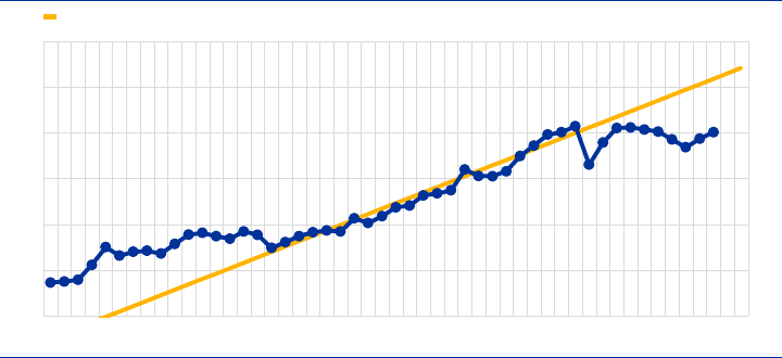
as not likely to turn to de-globalisation. The backward-looking part is illustrated in
Chart 1, which shows that after a period of very fast "hyperglobalisation" between the
mid-eighties and 2008, the share of world trade in world GDP has stayed roughly
constant.
Chart 1
World trade relative to world GDP (1970-2018)
Source: Antras (2021), based on World Bank’s World Development Indicators (link).
Note: Trade is defined as the sum of exports and imports of goods and services.
Looking forward, Antras argues that two out of three main factors that explained
"hyperglobalisation" are unlikely to reverse. First, new technologies will continue to
foster trade, as the case during the first Information and Communication Technology
(ICT) revolution, because those substituting (foreign) labour (such as robotisation or
3D printing) still generate increased demand for traded goods (such as machines or
IT parts). Second, the high sunk costs of establishing global supply chains make
them resilient to temporary shocks and make re-shoring only attractive for very
persistent shocks. The only hyperglobalisation factor risking to reverse is multilateral
trade liberalisation. So, in Antras' view the main challenges to globalisation are
political and institutional in nature. They can only be kept under control if
governments compensate the losers of globalisation better than they did in the past
(rather than resorting to protectionism).
10%
15%
20%
25%
30%
35%
40%
1970 1974 1978 1982 1986 1990 1994 1998 2002 2006 2010 2014 2018
Linear forecast based on 1986-2008 period
ECB Forum on Central Banking, November 2020
7
Susan Lund (in Lund 2021) added that China rotating from exports to domestic
consumption and building domestic supply chains can account for most of the global
trade slowdown over the last decade. As both reflect economic development, it may
be regarded as a positive story, one also other emerging economies may go through
in the future. Moreover, one should not forget that services trade grew much (about
80 per cent) faster than goods trade over a similar period. Lund, however, took a
somewhat different perspective on the resilience of global supply chains. Their
occasional disruption can have measurable implications for company profits and
therefore a large share of supply chain executives currently consider making them
safer, including through "near-shoring" and regionalisation.
Finally, Antras (2021) also discussed the impact of the COVID-19 pandemic on world
trade. His main conclusion was that, to the extent that economic agents perceive the
pandemic as a temporary shock (which has become more likely given the relatively
fast development of vaccines), the current crisis is unlikely to constitute a significant
de-globalisation force.
Climate change and the de-carbonisation that it requires is likely to set in motion
another set of major structural changes in the world economy, but Frederick van der
Ploeg (in van der Ploeg 2021) strongly warns that political logic involves the great
risk that too little is being done too late. This implies an unsmooth carbon transition
with financial market disruptions, stranded assets and financial instability. A sudden
shift in (expectations about) climate policy or a technological breakthrough can lead
to sudden changes in the market valuation of both carbon-intensive and carbon-
extensive firms (so-called tipping events).
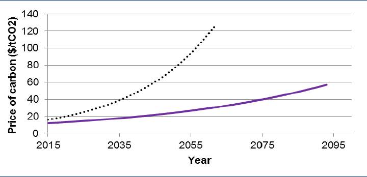
In his comprehensive survey paper, van der Ploeg first compares economists'
preferred Pigouvian approach of pricing carbon at its social costs (either via a carbon
tax or a system of tradable emission permits) with the route taken by the
Intergovernmental Panel on Climate Change (IPCC) of agreeing on a cap to global
warming. As illustrated in Chart 2 (taken from van der Ploeg 2018), the IPCC
approach would increase the carbon price (and therefore reduce carbon emissions
and increase renewables) much faster than standard Pigouvian approaches. The
Pigouvian approach doesn't take peak temperature constraints into account, and
thus prices don't have to rise so fiercely under it. In general, all these approaches
should not only curb the demand for fossil-fuel-based energy, but also stimulate
green research and development (R&D) and innovation, and speed up the move
towards a circular economy (in which resources are re-used rather than used up).
ECB Forum on Central Banking, November 2020
8
Chart 2
Evolution of the carbon price implied by the Pigouvian versus the carbon budget
approach to climate policy
Source: van der Ploeg (2018) and van der Ploeg (2021)
Note: The solid line represents the necessary evolution of the calibrated optimal carbon price, as derived from a simplified Dynamic
Integrated Climate-Economy (DICE, see e.g. Nordhaus 1993) model that sets the optimal price equal to the social cost of carbon
("Pigouvian approach"). The social cost is defined as the present discounted value of all future production losses stemming from
emitting one ton of carbon today. The dotted line not only takes into account the social cost of carbon but also the need to keep peak
global warming below 2 (relative to global temperature in the pre-industrial era; "carbon budget approach"). This is in line with the
route taken by the IPCC.
Among his many conclusions van der Ploeg (2021) calls for climate policies being
delegated to a politically independent emissions authority ("carbon central bank"),
the carbon price starting relatively high and then growing moderately but steadily
(avoiding paradoxical emission increases due to the anticipation of future policy
tightening), using revenues to compensate low-income households and to support
firms at risk from carbon-intensive imports, and using debt or transfers for
intergenerational fairness as well as keeping financial stability risks associated with a
disorderly transition under control with climate stress tests.
This stimulated a lively debate about the best institutional arrangements for
achieving timely decarbonisation. For example, Helene Rey wondered whether an
independent "carbon council" - as proposed in a recent Group of Thirty (2020) report
- could achieve net emissions neutrality by 2050 through targeting a carbon price
path and giving forward guidance in some analogy to independent central bank
monetary policy. Harald Uhlig cautioned not to overstretch delegation from
governments and parliaments to expert committees when re-distributional effects
induce some people to lose their jobs and some companies to go bankrupt. Lucrezia
Reichlin recalled that such active climate policies would still need much improved
and mandatory data standards and disclosure. Signe Krogstrup (in Krogstrup 2021)
wondered how one gets from van der Ploeg's literature overview suggesting that
climate risks are increasingly priced in financial markets to the under-pricing of risk
justifying policy intervention. In what concerns the role of central banks, Francois
Villeroy de Galhau suggested that central banks can look at whether climate risks
are adequately reflected in their collateral frameworks. Krogstrup concluded though
that fiscal policy should be first in line for a cost-efficient carbon transition, but central
banks will address their stake in it.
ECB Forum on Central Banking, November 2020
9
3 Formulations of central banks' inflation aim close to the
effective lower bound of nominal interest rates
One of the key challenges for monetary policy in our times is the sustained
downward trend in natural interest rates that can be estimated for the past decades
(see, e.g., Laubach and Williams 2003 on estimating the natural interest rate and
Brand et al. 2018 for euro area evidence). The low estimates of natural rates imply
that central banks' conventional interest rate policy may not be able to provide
sufficient stimulus in the presence of negative shocks, as policy rates cannot be
reduced low enough below the natural rate. This well-known problem gave rise to an
active discussion about the formulation of the ECB's inflation aim in its monetary
policy strategy.
In line with much of the New-Keynesian literature, Klaus Adam (in Adam 2021)
argued that an increase in the inflation target could be a solution, because - if the
increase is credible - the inflation expectations that it would induce would stimulate
the economy through lower real interest rates. But his research suggests that the
declining natural rate also influences asset price volatility and that therefore the
efficiency of financial markets has a bearing on the extent to which the target should
be increased and whether monetary policy should react to longer run asset price
fluctuations.
The New-Keynesian model developed in Adam et al. (2020) exhibits a negative
relationship between the natural rate and asset price volatility, as a lower discount
rate amplifies the present value changes of prices in response to future expected
pay-off changes. This relationship becomes more pronounced for inefficient
subjective price expectations (forecast errors are corrected sluggishly), as observed
in surveys, and therefore influences the level of the optimal inflation target. With
rational expectations in financial markets the optimal increase in the target to
compensate for the constrained policy rate is relatively small in the model. When
subjective expectations create procyclical asset price fluctuations, however, the
inflation target needs to be increased by much more, as the increased financial
volatility drives the economy more frequently towards the effective lower bound of
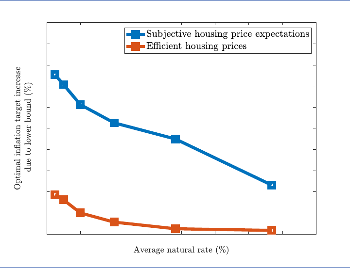
nominal interest rates (ELB). Chart 3 shows the optimal inflation targets (vertical
axis) derived from the model (calibrated to the US economy) for different levels of
the natural rate (horizontal axis) and depending on whether asset price volatility is
efficient (red line) or subject to procyclical adaptive behaviour emerging from
subjective expectations (blue line).
ECB Forum on Central Banking, November 2020
10
Chart 3
Relationships between the optimal inflation target, the natural rate of interest and
expectation formation in housing markets due to the effective lower bound on
nominal rates
Source: Adam (2021)
Note: This chart illustrates the optimal inflation target, i.e., the average inflation outcome under optimal conduct of monetary policy. For
each considered level of the average natural rate (on the x-axis), the chart reports the optimal inflation target (on the y-axis) in an
economy with an effective lower bound constraint, relative to the target that would be optimal in the absence of a lower-bound
constraint. The blue line shows the optimal inflation target in an economy where house prices are efficient (i.e. driven by fundamentals
only). The red line reports the optimal inflation target for the case where housing prices are driven – at least partly – by fluctuations in
subjective housing price expectations. Numbers are based on a New Keynesian sticky price model from Adam, Pfaeuti and Reinelt
(2020), calibrated to US data. In the absence of a lower bound constraint, the optimal inflation target is zero, because the model
abstracts from other forces that make targeting positive average rates of inflation optimal.
Interestingly, in this model the central bank finds "leaning" against inefficient asset
price fluctuations optimal, undershooting the inflation target in upturns and
overshooting it in downturns. The reason is that inefficiently high asset price volatility
has too high a welfare cost in terms of capital misallocation towards appreciating
assets.
In her discussion, Argia Sbordone (in Sbordone 2021) argued that, in Adam's model,
the increased incidence of the lower bound constraint does not imply that optimal
policy raises the long-term inflation target. Instead, it increases the number of
periods for which the central bank should temporarily target higher future inflation
than its stated long-term inflation target. This de facto would be similar to average
inflation targeting (AIT), the policy announced by the US Federal Reserve in 2020.
AIT makes up for past shortfalls in inflation relative to target through future inflation
that is temporarily in excess of the target. In Sbordone's view such a policy is
preferable, because it faces a lower risk of permanently higher inflation when ELB
incidences turn out to be infrequent. Alan Blinder made the point, however, that the
vague formulation by the Fed risked undermining the basic idea of AIT. Finally,
Sbordone pointed out that Adam's result about the optimality of "leaning against the
0 0.5 1 1.5 2 2.5 3 3.5 4
0
0.2
0.4
0.6
0.8
1
1.2
1.4
1.6
1.8
2
ECB Forum on Central Banking, November 2020
11
wind" is robust to various extensions of the model. In the context of the final panel of
central bank leaders, Federal Reserve Chairman Jerome Powell mentioned that the
Board of Governors took away from the fact that the 30-year long decline in inflation
and interest rates had contributed to financial imbalances and crises a very strong
focus on financial stability, as witnessed by its financial stability report published
since 2018.
In the first panel discussion Jordi Galí (in Galí 2021, Chart 1) showed a similar
negative relationship as Adam between the natural rate and the central bank's
optimal inflation target, based on a New-Keynesian model calibrated to euro area
data (Andrade et al. 2021). It suggests that while a target between 1.5 and 2 per cent
would be optimal for a steady-state real interest rate between 2 and 3 per cent, for
the lower equilibrium rate levels estimated nowadays the target could easily increase
to levels around 3 per cent. However, for increasingly aggressive monetary policy
rules embodying an AIT with rising averaging window to 4 or even 8 years, the
optimal target could be reduced to close to 2 per cent. Aggressive countercyclical
fiscal policy rules (e.g. emergency policies around 4 per cent of GDP in deep
recessions) would have a similar effect in the model. Galí concluded that rather than
deciding in favour of one of the three options, policy makers may want to pursue all
the three at the same time (although central banks can only control the first two).
Contributing additional perspectives to the discussion, Volker Wieland (in Wieland
2021) reached somewhat different conclusions. First, comparing average inflation
outcomes for the Harmonised Index of Consumer Prices (HICP, the ECB's headline
inflation indicator), the GDP Deflator and the Import Price Deflator, he argued that
the low inflation during the recovery after the European sovereign debt crisis seemed
to be mainly driven by import prices, which are hard to influence with monetary
policy, whereas the GDP deflator drifted towards levels above 2 per cent. Second,
the HICP does not capture owner-occupied housing, a category experiencing
significant price increases in some euro area countries. He therefore recommended
that the ECB would broaden the range of measures considered for its inflation
assessments. Next he presented elements of a model of optimal monetary policy in
which the effectiveness of unconventional monetary policies, such as quantitative
easing (QE), is subject to uncertainty and their adoption would have some
unintended side effects with welfare costs (Wieland 2020). Both considerations
would argue in favour of optimal monetary policies close to the ELB driving inflation
towards target more slowly rather than more aggressively, as e.g. suggested in the
AIT literature.
Overall, Wieland regarded it as problematic to raise the ECB's inflation aim at a time
when inflation is very low, as the distance between the two is very large in such a
situation and it would require further policy easing. If such easing is difficult to
achieve, the desired inflation expectations effect of a higher target may not
materialise and trust in the central bank’s ability to reach the target might be eroded.
In the general discussion, Vítor Constâncio and Ignazio Visco argued the other way
around, worrying that too little ambition could contribute to de-anchoring inflation
expectations making convergence to the desirable levels of inflation more difficult.
Yannis Stornaras wondered whether at the ELB expansionary fiscal policy was not
ECB Forum on Central Banking, November 2020
12
preferable to raising the inflation target. Adam and Galí recognised the challenge but
preferred to address it by revising the inflation target in smaller steps over time (e.g.
through regular reviews) and increasing it ("opportunistically") by more when inflation
has reached higher levels. Fabio Panetta drew from the discussion that central
banks have less conventional policy space for low inflation than for high inflation and
therefore have to act less tolerantly to inflation drifting below target.
4 Formal versus informal monetary policy communication
Annette Vissing-Jorgensen opened the topic of communication approaches for a
central bank's monetary policy strategy in her panel discussion (Vissing-Jorgensen
2021). While formal, public and on-the-record communications are a key and
unambiguously positive part of monetary policy making, ensuring its effectiveness
and accountability, the same does not apply to informal, off-the-record and
unattributed communications. And an academic literature using data for the United
States suggests that such informal communications - between meetings of the
Federal Open Market Committee - can have material effects on stock market returns.
Vissing-Jorgensen focused particularly on unattributed communications, such as
"sources stories" disseminated by the media. She recognised some benefits of such
informal communication if it is done institutionally, as non-attribution may preserve
more flexibility for policy makers, avoid time-consuming and potentially controversial
public debates and allow gauging outside views on different policy options. But she
regarded unattributed individual communication, driven by disagreements among
policy makers, as subject to a prisoner's dilemma-type problem and unambiguously
detrimental. She illustrated this point with a game-theoretic model of individual policy
makers trying to "spin" market expectations towards their preferred choices (Vissing-
Jorgensen 2020). While asset prices may not be distorted on average, as victories
and defeats cancel out over time, the policy space of the decision-making body will
still be constrained, as central banks have to mind about too frequent or large
deviations between market expectations and ultimate decisions. Apart from
discouraging individual unattributed communication, Vissing-Jorgensen
recommended consensus-building approaches for central bank governors, as they
would naturally reduce incentives for their committee members to engage in such
individual informal communications.
5 Monetary policy, the allocation of risk and central bank
independence
In the second panel discussion Lucrezia Reichlin (in Reichlin 2021) spelled out a
conceptual framework for the relationships between monetary policy, risk and
financial stability in the new world of unconventional instruments. Distinguishing what
she called "passive" instruments, such as long-term refinancing operations, which
act as complements to standard interest rate policy, from "active" instruments, such
as quantitative easing asset purchases, acting as substitutes for rate policy at the
ECB Forum on Central Banking, November 2020
13
ELB, she stressed the multi-dimensional use of the various instruments, which have
to be thought of as "packages" controlling the entire yield curve and creating
complex interactions between macroeconomic and financial risks.
These policies can only be effective in supporting the macroeconomy, if they induce
the creation of new assets climbing up the risk spectrum. If the new assets finance
productive activities, then the additional risks are "good". But prudential policy would
need to prevent the creation of "bad" risks. Delayed, partial or incoherent use of the
range of instruments would undermine effectiveness; and so would be neglecting
interactions and coordination with fiscal policy. In response to a question by Beatrice
Weder di Mauro, Reichlin emphasised the additional communication needs for
making the logic of the complex new instrument combinations and the
complementarities involved understood.
Hyun Shin (in Shin 2021) complemented this with emphasising the great importance
of "elastic nodes" in the financial system. In situations of stress, these elastic nodes
would flexibly accommodate the much-increased demand for money and thereby
help restore stability. The first line of defence should be well-capitalised and resilient
commercial banks; an example being how US banks increased commercial and
industrial loans during the "dash for cash" in March 2020, when the COVID crisis had
broken out, by allowing companies to draw on their credit lines. (In fact, several
Forum speakers - such as Jerome Powell and Bank of England Governor Andrew
Bailey - confirmed that banks generally stood up to this first major test of the reforms
introduced after the Great Financial Crisis.) Such elastic nodes are not new though,
as for example the strong deposit creation of the Bank of Amsterdam - an early
predecessor of central banks - through the acceptance of coins and bullion during
the crisis of 1763 illustrates (e.g. Schnabel and Shin 2004).
A third example of elastic nodes in the international arena is the circular flow of US
dollars between the Federal Reserve, the ECB, European and US-based banks
enabled through central bank swap lines. Its operation could be seen through a large
increase of cross-border interbank positions broadly matching the swap amounts
during the first quarter of 2020. So, central banks would constitute the second line of
defence, for example through facilities that Reichlin had included in her first category
of instruments complementary to conventional interest rate policy.
Markus Brunnermeier (in Brunnermeier 2021) broadened the discussion with a
proposal about how a monetary policy strategy can be robustified against the risk of
a central bank getting trapped in high inflation or deflation. At the time of the Forum
the main problem was still very low inflation. But in the post-COVID recovery an
"inflation whipsaw" could emerge, in that pent-up demand, government commitments
or capital re-allocation could create a reversal to high inflation (Brunnermeier et al.
2020). In other words, it is necessary that the central bank can "put on the breaks"
later, in order to be able to confidently stimulate the economy with force in the low
inflation context.
But if during the downturn government debt becomes too high, a situation of fiscal
dominance could occur, as the central bank could not raise interest rates in the
upturn without destabilising the budgets. Similarly, if the banking sector was not to
ECB Forum on Central Banking, November 2020
14
maintain its resilience and if the government was unwilling or unable to recapitalise
the banks, the central bank may be forced to stabilise them with monetary policy
redistributing risk - a situation of financial dominance.
Brunnermeier proposed that these tail risks, together with some other robustness
checks, would be considered in a re-oriented second pillar in the ECB's monetary
policy strategy. This would institutionalise heterogeneous thinking and go against
relying on a uniform class of economic models. Against fiscal dominance he
suggested to strengthen the central bank's independence through increasing its
equity capital. Against financial dominance Brunnermeier advocated adequate
prudential supervision and to design unconventional monetary policies in a way that
would not promote too much leverage in the financial and corporate sectors.
Paul de Grauwe challenged Brunnermeier on the need for re-capitalisations, as the
central bank can run monetary policy with negative equity and the creation of
additional central bank equity would not have any material macroeconomic
implications. Brunnermeier and Shin retorted, however, that there are limits for how
negative the central bank can go without the public's trust in the currency being
eroded (see also Hall and Reis 2015). Reichlin agreed and added that also the way
how seigniorage is distributed to treasuries may be relevant and it may be wise to
have some principles about that in the Eurosystem.
6 The role of fiscal policy in the post-COVID recovery
Evi Pappa (in Pappa 2021) made a strong plea for discretionary fiscal policy taking a
prominent role in the recovery from the COVID pandemic, notably through
government investment. The theoretical case relies on higher fiscal multipliers in a
situation in which conventional monetary policy is close to the ELB, as the central
bank would not tighten in response to inflation expectations ensuing from the fiscal
stimulus. In line with this, Christine Lagarde argued in her introductory speech to the
Forum (Lagarde 2021) that monetary policy should minimise any crowding out
effects on private investment that may emerge from rising market interest rates that
the fiscal expansion could induce.
Based on the experiences with European Union structural funds for member states
and regions over the last 30 years (see Canova and Pappa 2020, using a local
projections methodology), Pappa particularly supported public investment spending
funded by the Next Generation EU recovery programme (Table 1). For example,
grants provided by the European Regional Development Fund (ERDF), which aims
to foster investments in innovation and research, to foster the digital agenda, and to
support small and medium-sized enterprises, are found to have sizeable short-term
effects (over one year) on growth, investment, employment, productivity, and real
wages, making them particularly useful for rapid countercyclical policies. Measurable
effects of grants by the European Social Fund (ESF), whose aim it is to support
investments in education and health, and to fight poverty, take more time to
materialise (about three years). While these results mask strong cross-country
heterogeneity, countries like Finland, France, Italy, Latvia, Romania and Spain seem

ECB Forum on Central Banking, November 2020
15
to be systematically benefiting from the two funds in terms of growth and
employment. Accordingly, Lagarde (2021) called for the Next Generation EU
package to become operational without delay.
Table 1
Average cumulative multipliers from grants under the European Regional
Development Fund (ERDF) and the European Social Fund (ESF)
Macroeconomic
variables ERDF funds ESF funds
1 year 2 years 3 years 1 year 2 years 3 years
Gross value added
2.42
(0.19)
1.56
(0.32)
0.56
(0.32)
-0.14
(0.63)
2.70
(0.79)
5.05
(0.82)
Employment
0.86
(0.15)
-0.03
(0.27)
-0.42
(0.29)
-0.33
(0.23)
-0.62
(0.34)
0.96
(0.36)
Investment
8.07
(1.71)
0.53
(2.68)
-1.40
(2.69)
2.13
(1.65)
2.75
(1.63)
3.58
(1.88)
Labour
productivity
3.66
(0.37)
-3.65
(0.78)
-4.45
(0.75)
4.09
(0.70)
0.22
(0.83)
3.26
(0.85)
Real
Compensation
3.85
(0.36)
-2.62
(0.85)
-4.50
(0.84)
2.95
(0.32)
-1.54
(0.62)
4.54
(0.69)
Source: Canova and Pappa (2020)
Notes: This table examines the dynamic effects of ERDF and ESF grants on regional (NUTS3-level) macroeconomic variables in
European Union countries, using local projections. The main regression specification is as follows: y
,,
= a
,
+ b
,
y
,,
+ c
,
x
,,
+
e
,,
,where y
,,
is the cumulative growth of the macroeconomic variable of interest in region i and year t over the time-horizon h (either
1,2 or 3 years, see columns) and x
,,
is the cumulative change in the relevant grant (scaled by regional gross-value added). The
estimated coefficients displayed in the table correspond to c
,
and standard errors are in parentheses. The coefficients can therefore
be interpreted as the cumulative fiscal multipliers of the fund grants (euro change per euro of grants), or put differently as elasticities
measured in per cent, at each horizon h. Given the potential endogeneity of structural funds to EU economic conditions, the authors
instrument actual grants with their "innovations". To this effect they run the following auxiliary regression: x
,,
=
,
+
,
w
,
+ u
,,
,
where w
,
represents a set of four aggregate euro area variables: GDP, employment, the GDP deflator, the nominal interest rate, and
the nominal effective exchange rate. They then use the "innovation" u
,,
as an instrument for x
,,
in the main equation.
At the same time, Pappa cautioned that the literature suggests that the size of fiscal
multipliers can depend on many factors. For example, high public debt, low
confidence and economic uncertainty could reduce them or, in extreme cases, turn
them negative. While endorsing the proposals of the European Fiscal Board (2019)
for reforming the Stability and Growth Pact, she made the "daring suggestion" that
public debt restructurings in Europe may substantially ease the road to recovery (see
also Corsetti et al. 2016).
Vítor Gaspar (in Gaspar 2021) added that while national fiscal support packages
increased euro area public debt by about 17 percentage points during 2020 to above
100 per cent of GDP, the primary risk at the time of the Forum was the premature
withdrawal of fiscal support. Moreover, he joined Evi Pappa in supporting public
investment via the Next Generation EU programme, emphasising the International
Monetary Fund's assessment that fiscal multipliers are particularly elevated in
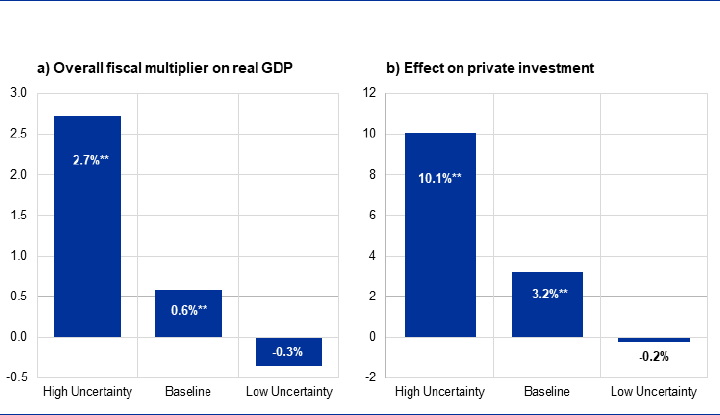
periods of high uncertainty (see Chart 5, based on IMF 2020), such as the case
during the COVID-19 pandemic (e.g. Barrero and Bloom 2020). According to Gaspar,
this happens because public support to investment in green and digital technologies
would facilitate and give confidence to private firms to invest, in part because public
investments signal governments' commitment to sustainable growth.
ECB Forum on Central Banking, November 2020
16
Chart 5
Public investment multipliers and private investment "crowd-in" for different levels of
economic uncertainty
Cumulative two-year-ahead macroeconomic effects of a one-percent-of-GDP unexpected
increase of public investment
Source: Gaspar (2021) and IMF Fiscal Monitor (October 2020)
Note: Effects on the vertical axes are measured in percentage changes. Results are based on local projection estimations using the
model y
,
y
,
=
+
+
G
,
FE
,
+
1 G
,
FE
,
+
,
+
,
, where y
,
is the log of the macroeconomic variable of
interest (real GDP for panel a) and private investment for panel b) for country i in year t, FE
,
is a positive unexpected shock to public
investment spending (as share of GDP), in deviation from IMF forecasts, z is an indicator of the degree of uncertainty, and G
,
is the
corresponding smooth transition function between different levels of uncertainty. M
,
includes lagged GDP growth and lagged shocks.
Uncertainty is measured by the standard deviation of GDP growth rate forecasts across professional forecasters as published by
Consensus Economics, using for each year the spring vintage of the forecasts. Data covers 72 advanced and emerging markets; the
sample period is 1994-2019.
The nuanced difference between Pappa and Gaspar on the role of uncertainty gave
rise to a discussion about which conditions would have to be fulfilled so that
multipliers remain positive (and potentially large) and the scope for multiple
equilibriums be reduced (as raised e.g. by Giancarlo Corsetti). Gaspar emphasised
investments in high-quality projects, high standards of transparency and governance
in infrastructure investments and a robust approach to public debt management.
Daniel Gros wondered whether containing uncertainty would not require addressing
public debt levels. Pappa mentioned the reduction of implementation lags, although
there could be a trade-off with quality. Moreover, the relative roles of fiscal and
monetary policy should be clearly communicated.
In her introductory speech, Christine Lagarde (in Lagarde 2021) had pointed out that
in a pandemic emergency, when interest rates are already very low, private demand
is constrained by health containment measures and levels of economic uncertainty
are very high, fiscal policy can be particularly effective for at least two more reasons.
First, it can support the sectors most affected in a more targeted way than monetary
policy (see also Woodford 2020). Second, as fiscal policy determines about half of
total spending in the euro area, it can help coordinate the other half, breaking
"paradox of thrift" dynamics in the private sector and thereby also reinvigorating the
transmission of monetary policy. All in all, the right policy mix requires that fiscal
policy remains at the centre of the stabilisation effort. At the same time, many Forum
speakers highlighted the unprecedented levels of uncertainty that the COVID
pandemic had generated and the challenges that it implied for the recovery. For
example, Andrew Bailey mentioned that relevant uncertainty measures reached
ECB Forum on Central Banking, November 2020
17
during 2020 their highest levels since a quarter of a century, making this feature the
most frightening aspect of the pandemic from an economic policy perspective.
References
Adam, K. (2021), “Monetary policy changes from falling natural interest rates”, in this
volume.
Adam, K., Marcet A., and Beutel, J. (2017), “Stock price booms and expected capital
gains”, American Economic Review, Vol. 107, pp. 2352-2408.
Adam, K., Pfaeuti, O. and Reinelt, Z. (2020), “Falling natural rates, rising housing
volatility and the optimal inflation target”, CRC TR 224 Discussion Paper, No. 235,
November.
Andrade, P., Galí, J., Le Bihan, H., and Matheron, J. (2021), "Should the ECB
Revise its Strategy in the Face of a Lower r*," mimeo., Pompeu Fabra University,
January.
Antras, P. (2021), “De-globalisation? Global value chains in the post-Covid-19 era”,
in this volume.
Attig, D., Baker, S., Barrero, J. M., Bloom, N., Bunn, P., Chen, S., Davis, S. J.,
Leather, J., Meyer, B., Mihaylov, E., Mizen, P., Parker, N., Renault, T., Smietanka, P.,
Thwaites, G. (2020), “Economic uncertainty before and during the COVID-19
pandemic,” Journal of Public Economics, Vol. 191, 104274.
Barrero, J. and Bloom, N. (2020), “Economic uncertainty and the recovery,” in
"Navigating the Decade Ahead: Implications for Monetary Policy", Federal Reserve
Bank of Kansas City, Economic Policy Symposium Proceedings, pp. 255-284.
Brand, C., Bielecki, M., and Penalver, A. (2018), “The natural rate of interest:
estimates, drivers, and challenges to monetary policy”, ECB Occasional Paper
Series, No 217, December.
Brunnermeier, M. (2021), “De- and inflationary traps: strengthening ECB’s second
pillar to avoid fiscal and financial dominance”, in this volume.
Brunnermeier, M., Merkel, S., Payne, J., and Sannikov, Y. (2020), COVID-19:
inflation and deflation pressures, mimeo., Princeton University, September.
Canova, F., and Pappa, E. (2021), “What are the likely macroeconomic effects of the
EU Recovery plan?”, mimeo., Pompeu Fabra UniversityFebruary.
Corsetti, G., Dedola, L., Jarocinski, M., Mackowiak, B. and Schmidt, S. (2016).
Marcoeconomic stabilization, monetary-fiscal interactions and Europe's monetary
union. ECB Working Paper Series, No 1988, December.
European Fiscal Board (2019), “Assessment of EU fiscal rules with a focus on the six
and two-pack legislation”. September 1.
ECB Forum on Central Banking, November 2020
18
Gali, J. (2021), “The decline in r* and the ECB strategy”, in this volume.
Gaspar, V. (2021), “Discussion of Evi Pappa’s “Fiscal rules, policy and
macroeconomic stabilization in the euro area””, in this volume.
Greenwood, R., and Shleifer, A., (2014), “Expectations of returns and expected
returns”, Review of Financial Studies, Vol. 27, pp. 714–746.
Group of Thirty (2020), "Mainstreaming the transition to a net-zero economy",
Washington (DC), October.
Hall, R., and Reis, R. (2015), "Maintaining central-bank financial stability under new-
style central banking ", mimeo., Stanford University, 16 July.
IMF (2020), Fiscal monitor: policies for the recovery, International Monetary Fund,
Washington. https://www.imf.org/en/publications/fm/issues/2020/09/30/october-2020-
fiscal-monitor.
Krogstrup, S. (2021), “Discussion of “Macro-financial implications of climate change
and the carbon transmission” by Frederick van der Ploeg”, in this volume.
Lagarde, C. (2021), "Monetary policy in a pandemic emergency", in this volume.
Laubach, T., and Williams, J. C. (2003). Measuring the natural rate of interest.
Review of Economics and Statistics, 85(4), pp. 1063-1070.
Lund, S. (2021), “De-globalisation? The recent slowdown of global trade and
prospects for future rebalancing”, in this volume.
Nordhaus, W. D. (1993), "Optimal greenhouse-gas reductions and tax policy in the
'DICE' model", American Economic Review, Vol. 83, pp. 313-317.
Pappa, E., (2021), “Fiscal rules, policy and macroeconomic stabilization in the euro
area”, in this volume.
Reichlin, L. (2021), “Non-standard monetary policy instruments: effectiveness and
risks”, in this volume.
Sbordone, A. (2021), “Discussion of “Monetary policy challenges from falling natural
interest rates” by Klaus Adam”, in this volume.
Shin, H.S. (2021), “Central bank balance sheets and financial stability”, in this
volume.
Schnabel, I., and Shin, H.S. (2004), "Liquidity and contagion: the crisis of 1763",
Journal of the European Economic Association, Vol. 2, pp. 929-968.
van der Ploeg, F. (2018), “The safe carbon budget”, Climate Change, Vol. 147, pp.
47-59.
van der Ploeg, F. (2021), “Macro-financial implications of climate change and the
carbon transmission”, in this volume.
ECB Forum on Central Banking, November 2020
19
Vissing-Jorgensen, A. (2020), " Central banking with many voices: the
communications arms race", mimeo., University of California at Berkeley, 2 February.
Vissing-Jorgensen, A. (2021), "Informal central bank communication", in this volume.
Wieland, V. (2020), “Quantitative easing: the proportionality principle and Brainard-
style policy attenuation”, unpublished manuscript., University of Frankfurt.
Wieland, V. (2021), “The decline in euro area inflation and the choice of policy
strategy”, in this volume.

ECB Forum on Central Banking, November 2020
20
Monetary policy in a pandemic
emergency
Introductory speech by Christine Lagarde
1
1 Introduction
Let me begin by welcoming all of you to this year’s ECB Forum on Central Banking.
Regrettably, we cannot be together in Sintra this time, but I trust that this virtual
environment will be no less conducive to challenging ideas and productive debate.
The purpose of this year’s conference is to examine the challenges facing central
banking in a shifting world. We will be discussing many of the long-term trends
monetary policy has to contend with, including shifting patterns of globalisation,
climate change and a lower natural interest rate.
Actually, the largest shift central banks are facing today may well turn out to be the
pandemic itself. As John Kenneth Galbraith said, “the enemy of the conventional
wisdom is not ideas, but the march of events”. And the events we are seeing today
are momentous.
The coronavirus (COVID-19) has produced a highly unusual recession and is likely
to give rise to a similarly unsteady recovery. Today I would like to talk about how the
ECB’s monetary policy has responded to this unique environment, and how we can
best contribute to supporting the economy going forward.
2 A highly unusual recession
The deliberate shutdown of the economy triggered by the COVID-19 pandemic has
produced a highly unusual recession. Most importantly, it has infiltrated and crippled
sectors that are normally less sensitive to the economic cycle. In a regular recession,
manufacturing and construction are typically hit harder by the cyclical downturn,
while services are more resilient. But during the lockdown in the spring, we saw the
reverse.
Compare our experience in the first half of this year with the first six months following
the Lehman crash. After Lehman, manufacturing contributed 2.8 percentage points
to the recession and services contributed 1.7 percentage points. But this year, the
loss was 9.8 percentage points for services and much less, 3.2 percentage points,
for manufacturing.
1
President of the European Central bank

ECB Forum on Central Banking, November 2020
21
This has three important implications.
First, research finds that the recovery from a services-led recession tends to be
slower than from a durable goods-led recession, as services create less pent-up
demand than consumer goods.
2
For example, people are unlikely to take twice as
many holidays abroad next year to compensate for their lack of foreign travel this
year.
Second, as services are more labour-intensive, services-led recessions have an
outsized effect on jobs. Five million people in the euro area lost their jobs in the first
half of this year. Of those, almost half worked in retail and wholesale trade,
accommodation and food services, and transportation, despite these activities
representing less than one-fifth of output. In the six months after Lehman, the worst
affected sector – industry – suffered only 900,000 job losses.
And third, these job losses hurt socio-economic groups unevenly. In the first half of
2020, the labour force contracted by almost 7% for people with low skills – who
typically also have lower incomes – while it fell by 5.4% for those with medium skills
and rose by 3.3% for those with high skills. This is double the loss of low-skilled jobs
we saw in the six months after Lehman.
In addition to their social impact, job losses for people with lower incomes present a
particular threat to the economy, because around half of those at the bottom of the
income scale face liquidity constraints and therefore consume more of their
income.
3
The labour-intensity of the worst-hit sectors also heightens the risk of
hysteresis and “scarring” in the labour market.
While job retention schemes have played a key role in mitigating these risks, they
could not eliminate them entirely. Even though many workers quickly returned to
regular employment once restrictions were lifted, a large number of people who lost
their jobs in the spring left the labour force and stopped looking for work, with 3.2
million workers classified as “discouraged”. This is so far different from the post-
Lehman period, when the drop in employment was matched by a rise in
unemployment.
And young people have been particularly affected, seeing disproportionate lay-offs
and delayed entry into the labour market. Research finds that this can have a variety
of long-lasting effects, including lower earnings ten to fifteen years later, and worse
future health conditions.
4
So, from the outset, this unusual recession has posed exceptionally high risks. That
is why an exceptional policy response has been required. And what has defined this
policy response, in Europe in particular, is the policy mix.
2
Beraja, M. and Wolf, C. (2020), “Demand Composition and the Strength of Recoveries”, mimeo.
3
Data from the ECB’s pilot Consumer Expectations Survey.
4
Von Wachter, T. (2020), “The Persistent Effects of Initial Labor Market Conditions for Young Adults and
their Sources”, Journal of Economic Perspectives, Vol. 34, No 4, pp. 168-194.

ECB Forum on Central Banking, November 2020
22
Learning the lessons of the last decade, there has been a renewed consensus that
the composition of policies matters for overcoming the crisis. More than ever before,
macroeconomic, supervisory and regulatory authorities have dovetailed and made
each other’s efforts more powerful.
3 Policy responses to the pandemic
What has this meant for monetary policy? There are two main ways in which we
have adapted the ECB’s policy to the pandemic: via the design of our tools and via
the transmission of our monetary policy.
First of all, we have responded to the unique features of the recession by designing
a set of tools specifically tailored to the nature of the shock, including recalibrating
our targeted longer-term refinancing operations (TLTROs), expanding eligible
collateral, and launching a new €1.35 trillion pandemic emergency purchase
programme (PEPP). The PEPP in particular has the dual function of stabilising
financial markets and contributing to easing the overall monetary policy stance,
thereby helping to offset the downward impact of the pandemic on the projected path
of inflation.
The stabilisation function of the PEPP is ensured by its flexibility, which is crucial
given the unpredictable course of the pandemic and its uneven impact across
economies. In this context, the PEPP’s flexibility allows us to react in a targeted way
and counter fragmentation risks. This was key in reversing the tightening of financing
conditions that we saw in the early days of the crisis.
In parallel, the stance function of the PEPP gives us the scope to counter the
pandemic-driven shock to the path of inflation – a path that has also been greatly
influenced by the specific characteristics of this recession. Not only has inflation
fallen into negative territory, but we have already seen services inflation, which is
normally the more stable part of the price index, drop to historic lows.
But the PEPP, together with the other measures we have taken this year, has
provided crucial support to the inflation path and prevented a much larger
disinflationary shock.
5
And its impact has been amplified by interactions with other
policies. For instance, the combined effect of the ECB’s monetary and supervisory
measures is estimated to have saved more than one million jobs.
6
At the same time, the nature of the pandemic also affects the transmission of
monetary policy. Normally, an easing of financing conditions boosts demand by
encouraging firms to borrow and invest, and households to bring forward future
5
Lagarde, C. (2020), “The monetary policy strategy review: some preliminary considerations”, speech at
the “ECB and Its Watchers XXI” conference, 30 September.
6
Altavilla, C., Barbiero, F., Boucinha, M. and Burlon, L. (2020), “The great lockdown: pandemic response
policies and bank lending conditions”, Working Paper Series, No. 2465, ECB, Frankfurt am Main,
September.

ECB Forum on Central Banking, November 2020
23
income and consume more. In turbulent times, monetary policy interventions also
eliminate excess risk pricing from the market.
But when interest rates are already low and private demand is constrained by design
– as is the case today – the transmission from financing conditions to private
spending might be attenuated. This is especially true when firms and households
face very high levels of uncertainty, leading to higher precautionary saving and
postponed investment.
7
In these circumstances, it is crucial that monetary policy
ensures favourable financing conditions for the whole economy: private and public
sectors alike. Indeed, these are the times when fiscal policy has the greatest impact,
for at least two reasons.
First, fiscal policy can respond in a more targeted way to the parts of the economy
affected by health restrictions. Research shows that, while monetary policy can
increase overall activity in this environment, it cannot support the specific sectors
that would be most welfare-enhancing. Fiscal policies, on the other hand, can
directly respond where help is most needed.
8
We have seen the efficacy of such targeting in the euro area this year. The ECB’s
Consumer Expectations Survey shows that households with lower income have seen
a greater reduction in the hours they work, but they have also received a higher
share of government support. As a result, while compensation of employees fell by
more than 7% in the second quarter, household disposable income fell by only 3%
9
,
because government transfers compensated for the loss of income.
Second, fiscal policy can break “paradox of thrift” dynamics in the private sector
when uncertainty is present. Public expenditure accounts for around 50% of total
spending in the euro area and can therefore act as a coordination device for the
other 50%. Our consumer survey demonstrates this: people who consider
government support to be more adequate display less precautionary behaviour. And
in this way, by brightening economic prospects for firms and households, fiscal policy
can help reinvigorate monetary transmission through the private sector.
4 The risk of an unsteady recovery
But regrettably the economic recovery from the pandemic emergency could well be
bumpy. We are seeing a strong resurgence of the virus and this has introduced a
new dynamic. While the latest news on a vaccine looks encouraging, we could still
face recurring cycles of accelerating viral spread and tightening restrictions until
widespread immunity is achieved.
7
Bloom, N., Bond, S. and Van Reenen, J. (2006), “Uncertainty and Investment Dynamics”, NBER
Working Paper Series, No 12383, National Bureau of Economic Research, July.
8
Woodford, M. (2020), “Effective Demand Failures and the Limits of Monetary Stabilization Policy”,
NBER Working Paper Series, No 27768, National Bureau of Economic Research, September.
9
Year-on-year changes.

ECB Forum on Central Banking, November 2020
24
So the recovery may not be linear, but rather unsteady, stop-start and contingent on
the pace of vaccine roll-out. In the interim, output in the services sector may struggle
to fully recover.
Indeed, services were already showing a declining trend before the latest round of
restrictions: the services PMI fell from 54.7 in July to 46.9 in October. And while
manufacturing has so far remained relatively resilient, there is a risk of the recovery
in manufacturing also slowing once order backlogs are run down and industrial
output becomes better aligned with demand.
In this situation, the key challenge for policymakers will be to bridge the gap until
vaccination is well advanced and the recovery can build its own momentum. The
strength of the rebound in the third quarter suggests that the initial policy response
was effective and the capacity of the economy to recover is still in place. But it will
require very careful policy management to ensure that this remains the case.
Above all, we must ensure that this exceptional downturn remains just that –
exceptional – and does not turn into a more conventional recession that feeds on
itself. Even if this second wave of the virus proves to be less intense than the first, it
poses no less danger to the economy.
In particular, if the public no longer sees the pandemic as a one-off event, we could
see more lasting changes in behaviour than during the first wave. Households could
become more fearful about the future and increase their precautionary saving. Firms
that have survived up to now by increasing borrowing could decide that remaining
open no longer makes business sense. This could trigger a “firm exit multiplier”,
where the closure of businesses faced with health restrictions cuts demand for
complementary businesses, in turn causing those firms to reduce their output.
10
If that were to happen, the recession could percolate through the economy to sectors
not directly affected by the pandemic – and potentially trigger a feedback loop
between the real economy and the financial sector. Banks might start tightening
credit standards in the belief that corporate creditworthiness is deteriorating, leading
to firms becoming less willing or able to borrow funds, credit growth slowing and
banks’ risk perceptions rising further. The ECB’s bank lending survey is already
signalling a possible tightening in the months to come. We are also seeing
indications that small and medium-sized firms are expecting their access to finance
to deteriorate.
A continued, powerful and targeted policy response is therefore vital to protect the
economy, at least until the health emergency passes. Concerns about
“zombification” or impeding creative destruction are misplaced, especially if a
vaccine is now in sight. Remember that lockdowns are a non-economic shock that
affects productive and unproductive firms indiscriminately. Policies that protect viable
10
Guerrieri, V., Lorenzoni, G., Straub, L. and Werning, I. (2020), “Macroeconomic Implications of COVID-
19: Can Negative Supply Shocks Cause Demand Shortages?”, NBER Working Paper Series, No
26918, National Bureau of Economic Research, April.

ECB Forum on Central Banking, November 2020
25
businesses until activity can return to normal will help our productive capacity, not
harm it.
The right policy mix is essential.
Fiscal policy has to remain at the centre of the stabilisation effort – the draft
budgetary plans suggest that fiscal support next year will be significant and broadly
similar to this year, and the Next Generation EU package should become operational
without delay. Supervisory authorities are working to ensure that banks can continue
to support the recovery by readying them for a potential deterioration in asset
quality.
11
And structural policies have to be stepped up so that policy support can
accompany the wide-ranging changes that the pandemic will bring, such as an
accelerating spread of digitalisation and a renewed focus on climate issues.
12
5 The outlook for monetary policy
So what is the role of monetary policy in this response?
It is clear that downside risks to the economy have increased. The impact of the
pandemic is now likely to continue to weigh on economic activity well into 2021.
Moreover, demand weakness and economic slack are weighing on inflation, which is
expected to remain in negative territory for longer than previously thought. This is
partially due to temporary factors, but the fall in measures of underlying inflation also
appears to be connected to the weakening of activity. And developments in the
exchange rate may have a negative impact on the path of inflation.
Continued policy support is therefore necessary to achieve our inflation aim. But we
should also consider how best to provide that support.
The unusual nature of the recession and the unsteadiness of the recovery make
assessing the inflation path harder than in normal times. Shifts in consumption
baskets caused by supply-side restrictions are creating significant noise in the
inflation data.
13
And the stop-start nature of the recovery means the short-term path
of inflation is surrounded by considerable uncertainty.
In these conditions, it is vital that monetary policy underpins inflation dynamics by
supporting demand and preventing second-round effects, where the negative
pandemic shock to inflation feeds into wage and price-setting and becomes
persistent. To that end, the best contribution monetary policy can make is to ensure
favourable financing conditions for the whole economy. Two considerations are
important here.
11
Enria, A. (2020), “Supervisory challenges of the pandemic and beyond”, speech at the Handelsblatt
European Banking Regulation Conference, 3 November.
12
Lagarde, C. (2020), “Remarks at the G30 International Banking Seminar”, contribution during the
session “Rebuilding and Sustaining Growth”, 18 October.
13
Kouvavas, O. et al. (2020), “Consumption patterns and inflation measurement issues during the
COVID-19 pandemic”, Economic Bulletin, Issue 7, ECB, November.
ECB Forum on Central Banking, November 2020
26
First, while fiscal policy is active in supporting the economy, monetary policy has to
minimise any “crowding-out” effects that might create negative spillovers for
households and firms. Otherwise, increasing fiscal interventions could put upward
pressure on market interest rates and crowd out private investors, with a detrimental
effect on private demand.
Second, monetary policy has to continue supporting the banking sector to secure
policy transmission and prevent adverse feedback loops from emerging. Firms are
still dependent on new flows of credit. And those that have borrowed heavily so far
need certainty that refinancing will remain available on attractive terms in order to
avoid excessive deleveraging.
In other words, when thinking about favourable financing conditions, what matters is
not only the level of financing conditions but the duration of policy support, too. All
sectors of the economy need to have confidence that financing conditions will remain
exceptionally favourable for as long as needed – especially as the economic impact
of the pandemic will now extend well into next year.
Currently, all conditions are in place for both the public and private sectors to take
the necessary measures. The GDP-weighted sovereign yield curve is in negative
territory up to the ten-year maturity. Nearly all euro area countries have negative
yields up to the five-year maturity. Bank lending rates are close to their historic lows:
around 1.5% for corporates and 1.4% for mortgages. And our forward guidance on
our asset purchase programmes and interest rates provides clarity on the future path
of interest rates.
But it is important to ensure that financing conditions remain favourable. This is why
the Governing Council announced last month that we will recalibrate our instruments,
as appropriate, to respond to the unfolding situation. The Council is unanimous in its
commitment to ensure that financing conditions remain favourable to support
economic activity and counteract the negative impact of the pandemic on the
projected inflation path.
In the weeks to come we will have more information on which to base our decision
about this recalibration, including more evidence on the success of the new
lockdown measures in containing the virus, a new set of macroeconomic projections
and more clarity on fiscal plans and the prospects for vaccine roll-outs.
While all options are on the table, the PEPP and TLTROs have proven their
effectiveness in the current environment and can be dynamically adjusted to react to
how the pandemic evolves. They are therefore likely to remain the main tools for
adjusting our monetary policy.
Looking beyond our next policy meeting, our ongoing strategy review gives us an
opportunity to reflect on the best combination of tools to deliver financing conditions
at the appropriate level, how those tools should be implemented, and what features
our toolkit needs to have to deliver on such a strategy.
ECB Forum on Central Banking, November 2020
27
6 Conclusion
Let me conclude.
The pandemic has produced an unusual recession and will likely generate an
unsteady recovery. All policy areas in Europe have responded promptly and
decisively. The European policy mix has proven that when different authorities work
together – within their respective mandates – countries can successfully absorb the
pandemic shock.
The second wave of COVID-19 presents new challenges and risks, but the blueprint
for managing it is the same. The ECB was there for the first wave and we will be
there for the second wave. We are, and we continue to be, totally committed to
supporting the people of Europe.
In pursuit of our mandate, we will continue to deliver the financing conditions
necessary to protect the economy from the impact of the pandemic. This is the
precondition for stabilising aggregate demand and securing the return of inflation to
our aim.

ECB Forum on Central Banking, November 2020
28
De-globalisation? Global value chains in
the post-COVID-19 age
By Pol Antràs
1
Abstract
Although the growth of international trade flows relative to that of GDP has slowed
down since the Great Recession, this paper finds little systematic evidence indicating
that the world economy has already entered an era of de-globalisation. Instead, the
observed slowdown in globalisation is a natural sequel to the unsustainable increase
in globalisation experienced in the late 1980s, 1990s and early 2000s. I offer a
description of the mechanisms leading to that earlier expansionary phase, together
with a discussion of why these forces might have run out of steam, and of the extent
to which they may be reversible. I conclude that the main challenge for the future of
globalisation is institutional and political in nature rather than technological. Zooming
in on the COVID-19 global pandemic, I similarly conclude that the current health
crisis may further darken the future of globalisation if it aggravates policy tensions
across countries.
1 Introduction
At the time of writing, the world is witnessing extraordinary events. The COVID-19
global pandemic has brutally awakened the world from a Panglossian tranquillity
caused by decades of relatively sporadic and largely isolated epidemic risks. The
magnitude and nature of the COVID-19 shock has quickly spilled over to the global
economy, triggering a dramatic decline in economic activity, due both to social
distancing practices but also due to government-mandated lockdowns and other
mobility restrictions.
In describing the unfolding and the consequences of the current COVID-19 health
crisis, journalists and commentators have been using the word “unprecedented” with
a frequency that is unprecedented. One example of such hyperbolic commentary is
the notion that the world economy has now entered a phase of de-globalisation in
which economic agents are increasingly severing their international economic links
1
Harvard University. This paper was written for the ECB Forum on Central Banking, “Central Banking in
a Shifting World,” originally scheduled to take place in Sintra, Portugal, in June 2020. I am grateful to
Jingyi Tao for outstanding research assistance, to Max Alekseev, Davin Chor, Evgenii Fadeev, Elhanan
Helpman, and Steve Redding for detailed comments, to Gita Gopinath and Şebnem Kalemli-Özcan for
helpful discussions, and to Diego Cerdeiro, Michael Clemens, Lionel Fontagné, Michele Mancini,
Sébastien Miroudot, and Josep Pijoan-Mas for sharing data with me. The author received an
honorarium for carrying out and presenting the research in this paper.

ECB Forum on Central Banking, November 2020
29
and are reshoring economic activity toward their domestic economies. Is the world
economy really getting de-globalised?
Ironically, such an unravelling of globalisation would not be unprecedented. The last
significant episode of de-globalisation occurred in the 20th century during the so-
called Interwar Period, a period which coincidentally witnessed at its onset one of the
most devastating global pandemics on record, the 1918 Influenza Pandemic.
2
Of
course, there are a myriad of forces that contributed to the de-globalisation of the
Interwar Period, none more important than (i) the belligerent and dysfunctional
political world order that emanated from World War I, and (ii) a worldwide economic
downturn – the Great Depression – that severely impacted many of the world’s
largest economies and led these countries’ governments to institute beggar-thy-
neighbour policies.
Luckily, the world has not witnessed a truly global military conflict since 1945. Yet the
Great Recession of the late 2000s brought to an abrupt halt the process of
globalisation that had begun in the post-war period and that had accelerated
remarkably in the mid-1980s. And, much as happened during the Interwar Period,
the recent Great Recession has rekindled nationalistic sentiments in many advanced
countries, fuelling a political rhetoric that blames foreigners for the economic woes
faced by the domestic residents of these advanced countries. Although the extent to
which this rhetoric has materialized into actual policies has been somewhat limited,
the recent trade disputes between the U.S. and China and the withdrawal of the
United Kingdom from the European Union have shaken the firm ground over which
the process of globalisation appeared to be cemented. To cap it all, since early 2020
the world economy has submerged itself into a global health crisis that, due to its
severity and asynchronous nature, has dramatically impacted the functioning of
global value chains.
In sum, in an era like the present one with significant health, economic and policy
uncertainty, it is natural that some commentators have spotted the beginnings of a
new era of de-globalisation.
3
The goal of this paper is to try to elucidate whether the
world economy might have indeed already entered such a phase of de-globalisation
and, more speculatively, to offer some thoughts on the future of global value chains
in the post-COVID-19 age.
The paper sets off, in section 2, by studying the process of globalisation in recent
decades. Unlike the view pushed by some commentators, the paper argues that
there is no conclusive evidence indicating that the world economy is significantly less
global today than it was at the onset of the Great Recession. It is certainly the case
that that pace of globalisation has slowed down relative to recent decades – a
process that The Economist has referred to as Slowbalisation
4
– but the anecdotal
2
Being a citizen of Spain, you will allow me to refrain from referring to the 1918 Pandemic as the
Spanish Flu, a denomination that is neither fair nor accurate.
3
See, for instance, the views voiced by economists, business leaders, and other experts interviewed in
“Have We Reached Peak Globalization?”, Bloomberg News, January 24, 2020 (link).
4
Economist. “Slowbalisation: The steam has gone out of globalisation.” The Economist (2019): 34-43
(link).
ECB Forum on Central Banking, November 2020
30
evidence based on individual firms’ decisions that is often mentioned to justify the
premonition of de-globalisation is not salient enough to show up in aggregate
statistics. The world trade-to-GDP ratio – a standard measure of globalisation – has
recovered from its late 2008 low, while last year, the share of migrants in world
population attained its highest level since 1990. The relative importance of capital
flows and multinational activity in overall economic activity has certainly gone down
since the Great Recession, but these series remain at high levels comparable to
those in the early 2000s. The same is true for the relative importance of global value
chain (GVC) trade in world trade.
Focusing on the evolution of the ratio of world trade to world GDP in the last fifty
years, I find that 80% of the growth in this ratio occurred during the subperiod 1986-
2008. Indeed, the ratio of world trade to world GDP almost doubled (increasing by a
factor of 1.72) during that period of “hyperglobalisation”. Because many measures of
globalisation are simple ratios or shares that have natural upper bounds, I argue that
growth explosions in trade openness of the type experienced during the
hyperglobalisation of 1986-2008 are simply not sustainable. In other words, a period
of “slowbalisation” was inevitable.
In order to elucidate why the process of globalisation slowed down, it is thus crucial
to study the forces that fuelled that earlier expansionary phase. I turn to this task in
section 3 of the paper. I identify three main developments beginning in the late 1980s
that led to a remarkable disintegration of production processes across borders. First,
the information and communication technology (ICT) revolution allowed firms in
industrialized countries to relocate certain parts of their production processes to
distant locations, while still maintaining a fluid flow of communication between the
different production units in GVCs, and also facilitated the design and
implementation of efficient supply-chain management practices. Second, this period
also witnessed a significant fall in effective trade costs, a reduction caused both by a
significant acceleration in the rate of reduction of man-made trade barriers (e.g.,
tariffs and other non-tariff barriers), and by the increased reliance on faster methods
of shipping goods, such as air freight shipping. Third, political developments in the
world – most notably the fall of communism in Eastern Europe and the gradual
increased adoption of market economy practices in East and Southeast Asia –
brought about a remarkable increase in the share of world population actively
participating in the process of globalisation.
In sum, at the same time that firms in industrialized countries found it easier and
cheaper to set up global value chains sustained by large flows of goods and
information across the globe, the world capitalist system witnessed a massive labour
supply shock, as hundreds of millions of workers (many of which were highly-
qualified workers) suddenly became “employable” from the point of view of firms in
these advanced economies. I close section 3 by developing a simple theoretical
framework to illustrate how these forces may have acted in independent but also in
complementary ways to generate a fast acceleration in the share of world trade
accounted for by global production networks. The framework also incorporates
imperfect competition and scale economies, and demonstrates the relevance of
scale for the decision of firms to slice their value chain across borders.
ECB Forum on Central Banking, November 2020
31
Having described some of the key forces that fuelled the hyper-globalisation of 1986-
2008, in section 4, I turn my attention to studying the extent to which these forces
might have run out of steam, and more importantly, to assessing the extent to which
they may be reversible. I first review some of the key technologies associated with
the ICT revolution and argue that, although the rate of technological change does not
seem to be slowing down for certain key technologies (e.g., Moore’s Law holds as
well today as it did in the 1980s and 1990s), sustaining such a pace of technological
progress requires increasingly high R&D outlays. Similarly, there are some signs of
diminishing returns in other technological developments that were crucial for hyper-
specialisation to take off. For instance, the number of internet users as a share of
world population is still growing but at a noticeably slower pace than in the 1990s.
Next, I reflect on the extent to which other new technologies that have only become
widely available in recent years might reduce rather than increase the profitability of
breaking up production processes. I first discuss the role of automation, which
constitutes an alternative to offshoring for firms in developed countries seeking to
lower their labour costs. Because automation and offshoring appear to be
substitutes, one might expect that future improvements in automation will naturally
lead to an increasing amount of reshoring over time, thus fuelling de-globalisation. A
similar case has been made regarding 3D printing. I argue, however, that both
conceptually as well as in light of recent empirical evidence, the de-globalising effect
of these technologies is much less clear-cut in practice. Furthermore, and as I review
in section 4, there are an array of novel, cutting-edge digital technologies that have
the potential to give hyper-globalisation a second wind in coming decades.
I conclude section 4 by returning to the conceptual framework developed at the end
of section 3. I argue that, even if the forces that led to hyperglobalisation might have
slowed down, and others might foster de-globalisation, the large economies of scale
associated with modern GVCs might make firms reluctant to dismantle them in the
face of severe but temporary shocks. More specifically, because firms incur large
sunk costs when putting in place their global sourcing strategies, their location
decisions are relatively sticky. I argue that this stickiness explains the fact that the
bulk of the trade collapse of 2008-09 occurred at the intensive (rather than
extensive) margin, thus sowing the seeds for the observed V-shape recovery in trade
flows in 2010. The lesson is that shocks to the world economy are likely to lead to
important changes in the geography of worldwide production only if these shocks are
large and perceived to be persistent.
Stepping away from technological factors, in section 5, I briefly study the potential
role of other secular long-term forces in potentially leading to a period of de-
globalisation. First, the labour supply shock associated with the transition of
communist and socialist countries into market economies will not go away, but unit
labour costs in less developed economies have grown considerably relative to those
in advanced economies, thereby eroding some of the benefits of fragmenting
production. I argue, however, that global value chains do not always seek low unit
labour costs, as reflected by the fact that an important share of GVC trade takes
place between advanced economies. Furthermore, given the sunk costs associated
with the current geography of worldwide production, it will take persistent and
ECB Forum on Central Banking, November 2020
32
significant shifts in competitiveness for firms to want to reshore activity to their own
domestic economies. In section 6, I also discuss the role of various types of
compositional factors. In particular, I show that investment rates appear to be going
down at the world level, and I argue that this might put downward pressure on
globalisation in the future, given the disproportionate importance of capital goods in
international trade flows.
Although the case for a process of de-globalisation based purely on technological
factors is somewhat weak, the risk of policy factors leading to an era of increased
isolationism deserves much closer attention. Are we on the cusp of a new Interwar
Period in terms of trade policy? Although the trade liberalization efforts of the post-
war period are certainly reversible, as Brexit or U.S.–China have vividly illustrated,
the effects of these novel policy distortions have been limited to date. Building on the
conceptual framework with sunk costs, I argue in section 6 that this tamed response
is largely explained by the fact that firms are uncertain about whether the restrictions
that have been put in place will be persistent. This leads me to study the underlying
forces that precipitated the globalisation backlash of the 2000s, in the hope of
elucidating the extent to which these forces will themselves be persistent. More
specifically, I discuss the role of trade-induced inequality and of the limited
compensation received by those that might have been negatively affected by the
hyperglobalisation of 1986-2008. I argue that technological progress in the coming
decades might not only give globalisation an extra push, but it might also aggravate
inequality. As a result, the political rhetoric that has fuelled the backlash against
globalisation will remain a challenge unless tax systems do a better job of providing
a safety net or offering active labour-market policies to those individuals
experiencing negative trade-related income shocks, such as job dislocations caused
by import competition.
In section 7, I turn to the current COVID-19 health crisis. I first document the effect it
has had on international trade flows. Government-mandated lockdowns in China led
to a first significant decline in trade flows in late January and in February of 2020,
with a disproportionate effect on international trade in vehicles (a canonical example
of GVC trade). After a recovery in early March, trade flows collapsed again in March
and April, with again a much larger response for “GVC” trade than for other types of
trade. Growth in world trade since May has been steady, however, and had virtually
reached early January levels by early September. Building on the conceptual
framework developed in section 3 extended to include sunk costs, I hypothesize that
the bulk of the response in the early phases of the pandemic was at the intensive
rather than the extensive margin. To the extent that economic agents perceive
COVID-19 as a temporary shock, I conclude that the current health crisis is not likely
to constitute a significant de-globalisation force in the near future. Nevertheless, I
anticipate two potential turns of events that could led to a more protracted negative
effect of the COVID-19 crisis on globalisation. First, whether the shock is permanent
or not is not yet entirely clear. At the time of writing a reliable vaccine is not yet
available, and there is the widespread perception that international business travel (a
key input in global production networks) will be disrupted for years to come. Second,
the negative externalities inherent in the spread of the disease across countries have
somewhat intensified the practice of “finger pointing” between countries, which is not

ECB Forum on Central Banking, November 2020
33
auspicious for a future easing of political tensions in coming years. Furthermore,
every indication at this point is that the current health crisis is likely to significantly
increase income inequality worldwide due to the differential ability of skilled and
unskilled individuals to work from home, and this again does not bode well for the
future of globalisation.
2 De-globalisation? The facts
In this section, I review the evolution of various measures of globalisation with the
goal of assessing whether the world economy has indeed entered a new era of de-
globalisation. Although the process of globalisation encompasses the integration of
goods, labour and capital markets, it is natural to begin our analysis with
international trade flows.
Chart 1 plots the evolution of the share of world trade over world GDP during the
period 1970-2018.
5
Several aspects of the figure are noteworthy. First, the ratio of
world trade to world GDP more than doubled, from an initial value of 13.7% in 1970
to 29.7% in 2018. Second, the bulk (close to 80%) of that increase occurred during
the twenty-three-year period between 1986 and 2008. Third, world trade openness
fell notably after the onset of the Great Recession, but it has since recovered and, in
2018, reached essentially the same level it had achieved at its peak in 2008.
Chart 1
World trade over world GDP (1970-2018)
Sources: World Bank’s World Development Indicators (link).
Does the time series in Chart 1 warrant the concern that the world economy might
have entered a phase of de-globalisation? The contrast between the
hyperglobalisation period 1986-2008 and the more recent period 2009-18 is certainly
noteworthy, but note that the period 1970-85 also saw a fairly restrained growth in
this ratio. More significantly, it is natural to imagine that in a world economy
converging to a balanced growth path, the ratio of world trade to world GDP will
stabilize to a constant steady-state value. In other words, one cannot possibly expect
5
World trade is defined as half the sum of world exports and world imports.
10%
15%
20%
25%
30%
35%
40%
1970 1974 1978 1982 1986 1990 1994 1998 2002 2006 2010 2014 2018
Linear forecast based on 1986-2008 period

ECB Forum on Central Banking, November 2020
34
the share of world gross output that is shipped across borders to grow without
bounds over time: it cannot possibly be higher than 100 percent!
6
An important caveat to this argument is in order. World GDP and world gross output
are two very different objects, and the ratio of world trade to world GDP could in
principle well exceed 100%, as it does for certain individual economies such as Hong
Kong or Singapore. Still, one would not expect the ratio of world GDP to world gross
output to grow at a constant rate in a balanced-growth path. This ratio has in fact
been quite stable at a value of one-half in recent decades (see Antràs and Chor,
2018).
In Chart 2, I explore the extent to which the observed growth in world trade in Chart
1 is associated with the emergence and consolidation of global value chains (GVCs).
There are many possible ways to measure the extent to which production processes
have become globalized in recent years. Borin and Mancini (2019) develop a natural
measure of the importance of GVC trade in total international trade. Building on
global Input-Output tables, they identify the share of a country’s exports that flow
through at least two borders.
7
These exports encompass two broad types of GVC
trade. On the one hand, GVC trade includes transactions in which a country’s
exports embody value added that it has previously imported from abroad. This type
of GVC participation is often referred to as backward GVC participation. On the other
hand, GVC trade also comprises transactions in which a country’s exports are not
fully absorbed in the importing country, and instead are embodied in the importing
country's exports to third countries. The latter form of GVC participation is often
dubbed forward GVC participation.
Chart 2
GVC trade as percentage of world trade
Sources: Borin and Mancini (2019), as reported in World Development Report (2020).
6
The upper bound is in fact lower than 100%. For instance, in a world with no intermediate inputs, if
bilateral trade flows are well approximated by a gravity equation then /1
(
/
)
. Using 2018 GDP figures for all countries in the world, this delivers an upper
bound for world openness of 90.1%.
7
See also Wang et al. (2013). Other important papers on the measurement of GVC participation include
the pioneering work of Hummels et al. (2001), Johnson and Noguera (2012), and Koopman et al.
(2014).
30%
35%
40%
45%
50%
55%
1970 1975 1980 1985 1990 1995 2000 2005 2010 2015

ECB Forum on Central Banking, November 2020
35
As Chart 2 indicates, according to the Borin-Mancini measure of GVC trade, the
overall share of GVC trade in total world trade grew very significantly during the
hyperglobalisation period 1986-2008, but it appears to have stagnated or even
declined since the Great Recession. A natural conclusion from Charts 1 and 2 is that
the hyperglobalisation of 1986-2008 was tightly related to the growth of global value
chains, while the slowdown since the Great Recession might also be related to a
slowdown in GVC activity.
8
As mentioned above, globalisation is a multi-faceted process that involves much
more than the flow of goods and services across countries. In Charts 3, 4 and 5, I
explore the evolution of three variables that are often associated with this process. In
Chart 3, I rely on data from the United Nations Population Division to report the stock
of international migrants in the world as a percentage of world population. Although
illegal immigration and the rise of refugees fleeing conflict might complicate the
interpretation of this figure, it is apparent that the stock of migrants as a share of
world population is at its highest level since 1990. When looking at individual regions
or countries, increases in the stock of migrants are observed across the board. For
instance, the share of migrants in total population grew from 6.9% to 10.9% in
Europe, and from 9.2% to 15.7% in the United States. In sum, despite a backlash
against immigration in several parts of the globe, there is little evidence that
migration flows have significantly slowed down or decreased in recent years. The
current COVID-19 pandemic and its associated travel restrictions have brought
migration flows to an abrupt stop, but the long-term consequences of this shock are
yet to be discerned, as I will discuss more extensively in section 7.
Chart 3
International migrant stock as percentage of world population
Sources: United Nations (link).
8
Due to the complexities in constructing global Input-Output tables, this data only becomes available
with a significant lag, so Chart 2 measures GVC trade only up to 2015. Despite their widespread use in
economic research, it is also important to emphasize two key limitations of global Input-Output tables.
First, because they rely on fairly aggregated Input-Output data, the resulting sectoral disaggregation of
GVC flows is pretty coarse. Second, in constructing them, researchers are forced to impose strong
assumptions to back out certain bilateral intermediate input trade flows that cannot be readily read from
either Customs data or national Input-Output tables (see de Gortari, 2019).
2.0%
2.2%
2.4%
2.6%
2.8%
3.0%
3.2%
3.4%
3.6%
1990 1995 2000 2005 2010 2015 2019

ECB Forum on Central Banking, November 2020
36
Chart 4 turns its attention to capital flows across countries as a measure of
globalisation. For both foreign direct investment and portfolio investment flows, it is
evident that the importance of these flows relative to world GDP peaked right before
the Great Recession and, by 2018, they were nowhere near to recovering from those
peak levels. Still, it is important to remember that the Great Recession was triggered
by the Global Financial Crisis of 2007-08, so it is perhaps less surprising that one still
observes some lingering effects of this crisis. This is for at least three reasons (see
Beck et al, 2020): (i) the Global Financial Crisis naturally resulted in persistently high
levels of risk aversion; (ii) the crisis led many governments to adopt macroprudential
policies that naturally restrained the inflow of capital into their economies, and (iii)
government bailouts provided an incentive for economic agents to lend in their
domestic economies, where the perceived (or conveyed) probability of being bailed
out was higher. Although the persistence of these factors might lead to a protracted
period of financial de-globalisation, this paper will not dwell too much on this set of
issues, since they fall well outside my expertise.
Chart 4
FDI inflows and portfolio investment inflows as a share of GDP (1970-2018)
Sources: Broner et al.’s (2013) World Bank Gross Capital Flows Data Files (link) and World Bank, WDI database for GDP (link).
Partly to alleviate concerns about the fickle nature of capital flows, in Chart 5 I study
the evolution of foreign direct investment from the operational (or real) side of
multinational companies. Building on data from the OECD (see also Cadestin et al.,
2018), I plot an estimate of the share of global output accounted for by foreign
affiliates of multinational corporations. Although the timeframe for this chart is more
limited than the one in the other charts in this section, the figure again suggests a
sizeable increase in the globalized nature of world production, followed by a marked
decline in the last ten years or so. Still, the relative contribution of foreign affiliates to
world output was larger in 2016 than in 2003. As in the case of the ratio of world
trade to world output, the remarkable increase in the early 2000s was clearly
unsustainable, and the decline in recent years points to a retrenchment in the
0%
1%
2%
3%
4%
5%
6%
7%
1970 1974 1978 1982 1986 1990 1994 1998 2002 2006 2010 2014 2018
FDI Inflows
Portfolio Investment Inflows

ECB Forum on Central Banking, November 2020
37
relative importance of GVCs comparable in nature to the evolution FDI inflows in
Chart 4 and of the share of GVC trade in world trade in Chart 2.
9
Chart 5
Foreign affiliates' gross output as a share of global output (2005-2016)
Sources: OECD, Analytical AMNE database (link
) for 2005-2016, and Cadestin et al. (2018) for 2000-04.
In sum, Charts 1 through 5 demonstrate that, although one could selectively pick
certain measures of globalisation to argue that the world economy has become de-
globalised since the Great Recession, world trade flows (as a percentage of world
GDP) are close to their all-time highest levels, and GVC and multinational firm
activity appear to have only retreated to their values in the mid-2000s. I conclude
that the evidence at this point is more consistent with the notion of “slowbalisation”
than with that of de-globalisation. Furthermore, in order to elucidate why the process
of globalisation might have slowed down and could potentially reverse, these five
charts suggest that it is paramount to study the forces that fuelled the expansionary
phase of 1986-2008. I turn to this task in the next section.
3 The period of hyperglobalisation
This section discusses some potential explanations for the extraordinary growth in
global value chain activity and international trade flows observed during the late
1980s, 1990s and early 2000s. Although many factors contributed to this growth, I
will highlight three particularly relevant developments: (i) the information and
communication technology (ICT) revolution, (ii) an acceleration in the rate of
reduction of trade costs, and especially trade costs associated with man-made trade
barriers, and (iii) political developments that brought about a remarkable increase in
the share of world population participating in the capitalist system.
9
Chart 2 plots the observations for the years 2000-04 in lighter blue because they are based on a
methodology that Cadestin et al. have improved upon since their 2018 working paper. I appreciate
Sébastien Miroudot’s guidance with this.
8%
9%
10%
11%
12%
13%
14%
2000 2001 2002 2003 2004 2005 2006 2007 2008 2009 2010 2011 2012 2013 2014 2015 2016
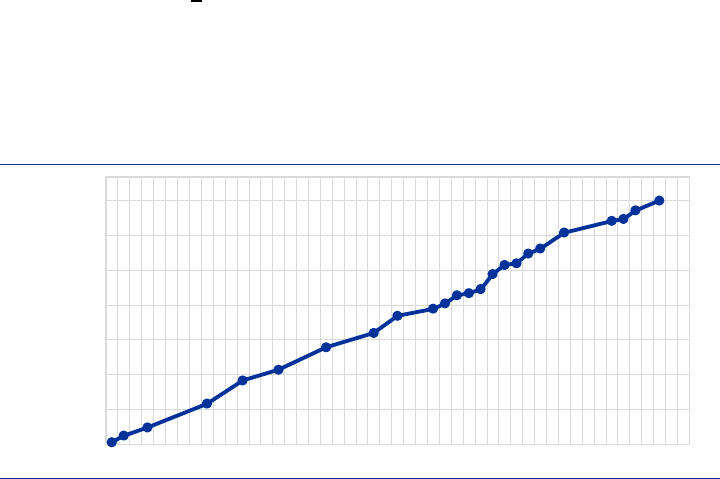
ECB Forum on Central Banking, November 2020
38
3.1 The ICT revolution
The 1980s and 1990s witnessed a genuine information and communication
technology (ICT) revolution that led to a profound socioeconomic transformation of
the world economy. Intel’s 386 microprocessor, released in 1985, had 275,000
transistors, achieved clock speeds ranging from 16 to 33 MHz, and was viewed as a
great feat of engineering. It sold for about $300 apiece. Only twenty-three years later,
in 2008, Intel introduced the iCore-7 microprocessor, which featured 731 million
transistors, a clock speed in excess of 3GHz, and sold at $284 apiece. This is not an
isolated example. The processing power and memory capacity of computers doubled
approximately every two years, as implied by Moore's law, and confirmed in Chart 6.
The almost perfectly linear fit in the graph features a slope equal to 0.384, which is
extremely close to
2
= 0.347.
Contemporaneously, the cost of transmitting a bit of
information over an optical network decreased by half roughly every nine months (a
phenomenon often referred to as Butter's law).
Chart 6
Moore’s Law: Number of transistors (log scale) per microprocessor (1971-2019)
Sources: Karl Rupp. 40 Years of Microprocessor Trend Data. Retrieved from Our World in Data (link).
Up to the mid-1980s, most internet networks were purpose-built, i.e. they were
intended for, and largely restricted to, closed communities of scholars. There was
hence little pressure for the individual networks to be compatible and, indeed, they
were largely not. International connections were relatively rare. Over the following
thirty years, the number of internet users increased by a factor of 600, from around
2.5 million users in 1990 to more than 1.5 billion users in 2008 (see Chart 7), which
amounts to a doubling of internet users roughly every two years.
2,000
20,000
200,000
2,000,000
20,000,000
200,000,000
2,000,000,000
20,000,000,000
1971 1975 1979 1983 1987 1991 1995 1999 2003 2007 2011 2015 2019

ECB Forum on Central Banking, November 2020
39
Chart 7
Number of Internet users as share of world population (log scale)
Sources: World Bank’s World Development Indicators (link).
As a result of these and other technological developments, the cost of processing
and transmitting information at long distances fell dramatically during the
hyperglobalisation period. The ICT revolution was thus instrumental for firms in
developed countries to contemplate the possibility of organizing and managing
production processes remotely. A salient example of this phenomenon is the
proliferation Computer-Aided Design And Manufacturing (or CAD/CAM), which
permitted the spatial separation of design and manufacturing, and has been shown
to have led U.S. companies to increase their use of contract manufacturing,
especially within the U.S., but also in distant foreign countries with a high enough
availability of skilled workers (see Fort, 2017).
The following thought experiment provides a final illustration of the transformative
nature of the ICT revolution. Try to envision how the world would have coped with
the current COVID-19 global pandemic without widespread access to powerful
computers and fast broadband internet connections. In case you need some help,
think about how, despite all their imperfections, video communications technology
companies such as Zoom have been instrumental in making it feasible for workers in
various types of occupations to work from home. Similarly, note how digital retailers
such as Amazon have facilitated social distancing practices by allowing individuals to
purchase many consumption goods from the comfort of their home.
3.2 The Golden Age of trade liberalization
During the same period, 1986-2008, governments intensified their efforts to gradually
dismantle the man-made trade barriers that were erected in the 20th-century’s
Interwar Period. This process dates back to the initial signing of the General
Agreement on Tariffs and Trade (GATT) in 1947, but experienced a revitalization in
the 1990s and 2000s with the signing of several notable regional trade agreements.
The European Community granted accession to Spain, Portugal and Greece in
1986, and its offspring, the European Union, was later enlarged to include several
East European countries in the 2000s. In the Americas, the early and mid-1990s saw
the formation of the North American Free Trade Area (NAFTA) between the U.S.,
0%
0%
1%
10%
100%
1990 1992 1994 1996 1998 2000 2002 2004 2006 2008 2010 2012 2014 2016
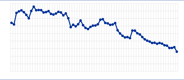
ECB Forum on Central Banking, November 2020
40
Canada and Mexico, and the Mercosur trade bloc in the Southern hemisphere. In
Asia, the ASEAN free trade agreement of 1992 and its later expansions created a
trade bloc of 10 East Asian nations. In parallel to this process of regional trade
integration, the WTO continued its program of multilateral trade liberalization by
lowering MFN tariffs (with the Uruguay Round concluding in 1994 with the creation of
the World Trade Organization) and by granting access to new members. In the latter
sense, China's accession to the WTO in 2001 was a particularly historic event.
Chart 8 demonstrates that, as a consequence of this wave of trade agreements, the
world’s weighted average tariff applied on traded manufactured goods fell
precipitously from 13.6% in 1986 to 7.5% in 2008. Interestingly, this trend does not
appear to have reversed since the Great Recession, as the unweighted world
average tariff had fallen additionally to 5.2% by 2017.
A noteworthy aspect of the process of trade liberalization is that it not only reduced
the average level of tariffs, but it also reduced trade-policy uncertainty due to the
binding commitments that countries made when entering the GATT/WTO or signing
regional trade agreements. In other words, not only were tariffs reduced on impact,
but there was also the general sense that the institutions being put in place would be
effective in precluding the reinstatement of protective trade measures (see Pierce
and Schott, 2016, Handley and Limao, 2017).
Beyond the gradual removal of man-made trade barriers, the 1980s and 1990s also
witnessed technological developments that significantly reduced the quality- and
time-adjusted costs of transporting goods across countries, in large part due to the
increased reliance on air freight shipping (see Hummels, 2007). For certain
industries (such as the hard disk drive industry), whose value chains rely on
continuous shipments of parts and components featuring high value-to-weight ratios,
the time saving associated with air shipping effectively constituted a large decline in
the cost of organizing their value chains at the global level.
Chart 8
Unweighted world average tariff (1950-2017)
Sources: Clemens and Williamson (2004) for the period 1950-1998 and World Bank’s World Development Indicators (link) for 1999-
2017.
0%
2%
4%
6%
8%
10%
12%
14%
16%
18%
1950 1955 1960 1965 1970 1975 1980 1985 1990 1995 2000 2005 2010 2015

ECB Forum on Central Banking, November 2020
41
3.3 The spread of capitalism
The third main lever of GVC growth during the hyper-specialisation era was
institutional in nature. Political developments in the world brought about a
remarkable increase in the share of world population that could feasibly participate in
the process of globalisation. In Europe, prior to 1989, millions of workers in the
Eastern part of the continent, many of them highly skilled, waited for better economic
opportunities behind an “iron curtain” instituted by communism (and enforced by the
Soviet Union). In China, the transition to a socialist market economy only began in
1978, when Deng Xiaoping introduced his programme of “socialism with Chinese
characteristics,” and foreign investment started pouring in soon after, exploding in
the 1990s. Similarly, in 1991, India initiated a process of economic liberalization that
eventually turned the country into a free-market economy.
Table 1
Share of world population of selected socialist countries in 1990
China 21.5% East Germany 0.3%
India 16.5% Hungary 0.2%
Bangladesh 2.0% Czech Republic 0.2%
Vietnam 1.3% Bulgaria 0.2%
Poland 0.7% Serbia 0.1%
Romania 0.4% Slovak Republic 0.1%
Sources: World Bank’s World Development Indicators (link) and Statistiches Bundesamt for East German data (link).
Table 1 provides information on the share of world population in 1990 accounted for
by ten selected countries that were socialist at that point in time and that have
become deeply ingrained in global value chains in recent decades. Together, they
accounted for to 43.5% of world population in 1990. The sheer size of this labour
force implies that, at the same time that firms in advanced economies recognized the
increased possibility of fragmenting production across borders and thus increased
their demand of “foreign” labour, the capitalist system witnessed a massive labour
supply shock that permitted Western firms to fulfil their demand without quickly
bidding up the price of foreign labour.
It should also be pointed that, even in capitalist countries, during this period there
was a noticeable ideological shift to the right in policy making, as exemplified by
Ronald Reagan’s presidency in the U.S. and Margaret Thatcher’s three terms as
Prime Minister of the United Kingdom. Thus, not only did former communist and
socialist countries embrace mainstream capitalist policies, but these policies
themselves became more friendly towards globalisation, as exemplified by the
deepening of trade liberalization described in section 3.2, but also by a notable
relaxation of currency convertibility and balance of payments restrictions in several
low and middle-income countries.

ECB Forum on Central Banking, November 2020
42
3.4 Why these forces mattered: a simple conceptual framework
Having loosely described the potential relevance of the ICT revolution, trade
liberalization, and the expansion of the “capitalist labour force”, I next develop a
simple theoretical framework (building on Antràs, 2003, and Antràs and Helpman,
2004) to more formally study the role of these three phenomena in explaining the
spectacular increase in the growth of GVCs.
Imagine a simple world with just two countries, an advanced West and a developing
East. We will largely be concerned with how a firm headquarted in the West
organizes the production of a certain good, which is only consumed in the West. For
now, it is assumed that production requires only two stages of production: (i)
headquarter services denoted by ; and (ii) manufacturing production, denoted by .
We will assume that these stages are used in fixed proportions, with a unit of output
requiring
units of headquarter services and
units of manufacturing production.
Headquarter services can in principle be produced in either country, but we shall
assume that the West has a strong enough comparative advantage in the provision
of these services to ensure that they are always produced in the West. We denote
the marginal cost of headquarter services by
, though this variable will not play an
important role in the analysis below.
Manufacturing production is carried out by workers and can be done in either the
West or the East. When done in the West, the firm needs to hire one worker per unit
of manufacturing output at a cost . It is assumed that because the other stage of
production, headquarter services, is always performed in the West, the firm need not
incur any additional marginal costs, such as shipping or trade taxes when
manufacturing is also carried out in the West. When producing in the West, the firm
thus faces an overall marginal cost of production equal to
+
.
When instead a firm chooses to internationally fragment production by moving the
manufacturing stage to the East, the Western firm is assumed to require hiring
1
workers per unit of manufacturing output at a cost
, where
< . In words, we
assume that workers in the less-developed East command a lower wage, but they
are also (weakly) less productive than their Western counterparts. In addition, the
firm’s marginal cost when manufacturing in the East is inflated by ad-valorem
communication costs
> 1, shipping costs
> 1, and tariffs
> 1. When
fragmenting production by manufacturing in the East, the firm thus faces an overall
marginal cost of production equal to
+
.
10
This marginal cost will
be lower than the one associated with the whole production process staying in the
West whenever
< . (1)
10
We are implicitly assuming that the good manufactured in the East is shipped back to the West, where
it is combined with headquarter services into final assembly and distribution. It would be straightforward
to study the case in which the good is instead assembled in the East, so transport costs are instead
associated with shipping headquarter services from the West to the East, and with shipping the final
good back to the West.

ECB Forum on Central Banking, November 2020
43
As equation (1) makes clear, the firm will only be able to reduce its marginal cost by
offshoring whenever Eastern productivity-adjusted wages are low, whenever
communication costs are low, and whenever transportation costs (i.e., shipping costs
and tariffs) are low. This equation thus illustrates very simply the relevance of the ICT
revolution described in section 3.1 (a reduction of
) and of the reductions in trade
costs documented in section 3.2 (indicating lower values for
and
).
11
Furthermore, it is also natural to interpret the spread of capitalism to Eastern Europe
and to Southeast Asia as the emergence of a new “Eastern” labour force offering
lower unit labour costs (lower
) to Western firms contemplating offshoring
manufacturing production to the East.
I have so far focused on a discussion of the marginal costs associated with different
locations of manufacturing. Yet distinct global value chain strategies naturally also
entail different levels of fixed (or overhead costs) associated with the corresponding
location choices of production.
12
Let us then incorporate fixed costs associated with
setting up manufacturing production units, with the natural assumption that the fixed
cost is larger when setting the plant up at a distance (i.e., in the East) than in the
West, or
>
, where is associated with domestic manufacturing and with
offshore manufacturing. Antràs, Fort and Tintelnot (2017) indeed estimate fixed costs
of global sourcing that increase in distance with an elasticity of around 0.2 for U.S.
manufacturing firms in 2007. I also assume that the firm has some degree of market
power, both because this is a realistic assumption and because it will allow firms to
cover the fixed costs of production by charging a mark-up over marginal cost.
Adopting the monopolistic competition cum love-for-variety-CES preferences that is
standard in the international trade field, we can express operating profits as a simple
function of the marginal cost to a negative power –
(
1
)
, where is the price
elasticity of demand faced by the firm.
13
The condition for the firm to want to offshore
manufacturing is now hence given by:
(
+
)
(
)
>
(
+
)
(
)
, (2)
where is a term associated with the level of demand faced by the firm, which is in
turn positively affected by how much consumers value the firm’s output and
negatively affected by competition from other firms in the industry.
Equation (2) confirms the role of foreign marginal labour costs, communication costs
and trade costs in shaping the profitability of offshoring vis à vis domestic
manufacturing. The main novel insight from equation (2) is that even when the
condition in equation (1) is satisfied, a firm may not find it profitable to offshore if the
difference
is large and if the scale of the firm is not sufficiently large. In
11
Note that the ICT revolution also potentially reduced trade costs
due to the role of technology in
enhancing the efficiency of supply-chain management.
12
As I have emphasized in my own work, marginal and fixed costs of production associated with different
configurations of global value chains may also be shaped by the organizational decisions of firms, most
notably, by whether they internalize foreign production processes or not (see Antràs, 2015, for a
review).
13
This formulation originates in the work of Dixit and Stiglitz (1980) and became mainstream in the trade
field with the work of Krugman (1980) and Melitz (2003), among many others.

ECB Forum on Central Banking, November 2020
44
words, because offshoring entails higher scale economies than domestic production,
it will typically be a strategy that only sufficiently large firms can profitably sustain.
14
It is also interesting to study a variant of the model in which the production process
entails several production stages rather than just two. In particular, imagine that
manufacturing production encompasses distinct production stages, each leading
to a distinct component, with the components then combined with headquarter
services to assemble the final good in the West. The firm now faces the choice of
whether to offshore or produce domestically each of these components. Assuming
that final good production entails
units of headquarter services and
units of
each of the manufacturing components = 1, … , we can express profits of a given
global value chain strategy as:
=
+
+
×
(
)
×
(
)
(3)
In this expression,
is an indicator function taking a value of 1 when component is
offshored, and a value of 0 when it is sourced domestically. Note also that we allow
cross-input heterogeneity in the extent to which transport costs and communication
technologies affect the productivity of foreign labour versus domestic labour.
As Antràs, Fort and Tintelnot (2017) stress, this multi-input variant of the model
illustrates the presence of interesting complementarities in the global sourcing
strategies of firms. Technically, whenever
< , the profit function in (3)
features increasing differences in (1
, 1
) for all , {1, . . . , } and . This result in
turn implies that the marginal benefit (in terms of firm profits) of offshoring any
component can only be increased by the decision of the firm to offshore some other
component .
15
Intuitively, whenever offshoring reduces marginal costs, firms will
increase their optimal scale of operation, and this will put them in a better position to
amortize the fixed costs associated with further investments in offshoring. This result
provides an amplification mechanism that helps explain, for instance, the magnified
response of gross trade flows to observed changes in trade costs (see also, Yi,
2003). It is also consistent with the notion that the combination of improvements in
communication technologies, trade liberalization and the adoption of market
economy practices in socialist countries produced a combined effect on the
geography of worldwide production that was larger than the sum of the individual
effects that these forces would have had in isolation.
16
14
Although the residual demand level is endogenous to the industry equilibrium associated with the
model, its determination would not undo the comparative statics described above. For instance, when
all firms are identical, it is easy to invoke a free-entry condition to show that all firms will offshore when
is sufficiently low, and they will all manufacture domestically when this composite foreign
cost term is high.
15
Clearly, if
> no firm would find it profitable to offshore that component , so the result is
irrelevant for that set of inputs.
16
The above complementarity relies on the degree of substitution of inputs being low relative to the
elasticity of demand faced by the firm. This condition is naturally met when inputs are perfect
complements, as in the simple model above, but the result generalizes to higher degrees of input
substitutability and is consistent with empirical evidence (see Antràs, Fort and Tintelnot, 2017).
ECB Forum on Central Banking, November 2020
45
Another implication of introducing fixed costs of offshoring is that they naturally lead
to rationalisation in the global sourcing strategies of firms. Although firms would
prefer to rely on several suppliers to obtain a given component – both for
diversification purposes as well as to extract a more favourable price – in practice
multi-sourcing involves fixed costs that are too large for most firms to bear (see
Antràs, Fort and Tintelnot, 2017).
I close this section with a final extension of the model, inspired by the work of Antràs
and de Gortari (2020), that illustrates the relevance of the sequential nature of
production in many GVCs. I again consider the case of multiple manufacturing
components, but I now assume that they need to be produced in a deterministic
order dictated by engineering constraints. At each stage, the producer of that stage’s
component combines labour and the good produced up to the prior stage in fixed
proportions. For simplicity, I assume that there are only two components = 1 and
= 2, that there are no frictions to communication nor any shipping costs across
countries (so
= 1), and that the inputs are fully symmetric except for their
position in the GVC. In terms of its location decisions, the firm thus only decides
whether to offshore component 1, component 2, both, or neither. The profit function
associated with each of these potential global sourcing strategies can be compactly
expressed as:
=
+
+
(
1
)
(
1
)
+
+
(
+
(
1
)
)
2
(
+
)(
)
Note that the third marginal cost term associated with the second stage is
unchanged relative to the case of multiple (but non-sequential) components, but the
one associated with the first stage is more involved. The reason for this is that profits
depend not only on production costs, but also on the total transport costs associated
with each particular path of the global value chain. To demonstrate the implications
of this feature, notice that if stage 2 is produced in the West (
= 0), then the first
stage will be offshored to the East only if
< /
, while if stage 2 is produced in
the East (1
= 1), the first stage will be offshored to the East only if
<
. The
latter is obviously a weaker condition than the former. In sum, trade costs and
sequentiality of production give rise to complementarities in the co-location of inputs
that may again lead to interesting interdependencies across the offshoring decisions
of firms, with the potential to explain the remarkable growth in offshoring during the
period of hyper-specialisation (see also Baldwin and Venables, 2013).
As mentioned in section 3.3, the hyperglobalisation of the 1980s, 1990s and early
2000s brought about not only an accelerated process of trade liberalization but also
a relaxation of constraints on the free mobility of capital across countries. It is natural
to imagine that this mechanism also contributed to the growth of offshoring by
reducing the cost of capital in countries that were eager to host GVC activity.
Although it would be straightforward to add physical capital to the model to capture
this force, the static framework developed above is admittedly too crude to capture
the role of financial capital flows in GVC activity.
ECB Forum on Central Banking, November 2020
46
4 De-globalisation and technological factors
Having developed a better understanding of some of the key forces that led to the
process of hyper-globalisation of the late 1980s, 1990s and early 2000s, I next turn
to assessing why these factors might have run out of steam in the last ten years and,
more importantly, to speculating on the extent to which they might be reversible. This
section will focus on technological factors, while sections 5 and 6 will cover other
long-term factors and political/institutional factors, respectively.
4.1 Is the ICT revolution over?
As discussed in section 3.1, the hyper-globalisation period witnessed the advent of a
series of technological developments that revolutionized manufacturing and
facilitated the fragmentation of production across countries. Is the slowdown in world
trade associated with a slowdown in the pace of technological progress? I do not
intend to provide a thoroughly researched answer to this question, but the almost
perfect fit in Chart 6 up to 2018 is highly suggestive that the pace of technological
progress in semiconductors has not slowed down. Furthermore, we continue to
witness ever increasing speeds of information transmission over fiber optic cables.
Nevertheless, it also seems intuitive that the marginal benefit of these innovations for
the international organization of production might have reached diminishing returns.
Being able to transmit information at long distances was crucial at the onset of the
phenomenon, but once the internet achieved high enough speeds to sustain smooth
communication for international production teams (e.g., via videoconferences), the
return to further improvements in these technologies is likely to have gone down.
Similarly, it is also important to point out that the amount of R&D spending required
to sustain Moore’s Law is much higher today than it was in the 1970s and 1980s
(see Bloom et al., 2020).
Chart 7 is also revealing in this respect. Although the diffusion of the internet still has
a long way to go (the World Development Indicators estimate that only 49% of the
world population used the internet in 2017), this Chart shows that the rate of
increase of internet adoption has significantly slowed down in recent years, as one
would have expected from the fact that this share cannot possibly be higher than
100%.
4.2 A new technological revolution?
Perhaps the key drivers of the ICT Revolution might have slowed down over time,
but a more intriguing possibility relates to the extent to which new technologies that
have become widespread in recent years might prove to be more conducive to de-
globalisation than the technologies that fuelled the ICT Revolution.
The example of industrial automation and robotics is a case in point. At first glance,
automation constitutes an alternative to offshoring for firms in advanced economies
seeking to lower their labour costs. Because automation and offshoring appear to be
ECB Forum on Central Banking, November 2020
47
substitutes, one would then expect improvements in automation to lead to an
increasing amount of reshoring over time. Furthermore, large multinational
companies typically design their production processes with their domestic market
factor prices in mind, so even when they engage in offshoring they might set up
manufacturing processes involving large amounts of automation in their host
countries (see Rodrik, 2018). This phenomenon is particularly concerning for less
developed economies, which might view automation as a threat to their ability to
leverage their cheap labour to get a foot in the door of GVCs.
Nevertheless, the substitutability between automation and offshoring is much less
clear-cut in practice. Automation by firms in advanced economies tends to decrease
their costs, enhance their productivity and increase their optimal scale, thereby
increasing their demand for intermediate inputs, many of which continue to be
sourced from less developed economies. Whether automation increases or reduces
the extent to which firms in less developed economies participate in GVCs is thus an
empirical matter. Artuc et al. (2018) and the World Development Report (2020,
Chapter 6) present industry-level evidence suggesting that automation in industrial
countries appears to have, in fact, boosted imports from developing countries. In
more recent work, Stapleton and Webb (2020) have confirmed these findings with
much richer firm-level data from Spain, while Wang (2020) is currently exploring the
same mechanism using detailed U.S. Census data.
Conveniently, it is relatively straightforward to illustrate the potential complementarity
between automation and offshoring with the conceptual framework developed in
section 3.4 (see also Wang, 2020). In particular, consider the version of the model
with multiple inputs and non-sequential production, but now expand the range of
strategies available to firms by giving them access to the possibility of automating
stage at a fixed cost
>
, which allows manufacturing of stage in the West at
cost
< . With this assumption, the profit function of Western firms becomes
+
+
×
×
(
)
+
×
×
(
)
×
(
)
×
(
)
.
In this expression,
is an indicator function taking a value of 1 when component
is automated and 0 otherwise. Focusing on a particular component i, it is clear that
the new possibility of automation reduces the range of parameter values for which
offshoring will be optimal. But because automating component i reduces marginal
costs and thus increases the optimal scale of the firm, it is also the case that the
probability that offshore-manufacturing dominates non-automated domestic
manufacturing is increased for components satisfying
< . In sum, the
automation of certain stages of production may well increase the demand for
offshore components that are harder to automate, and may well increase the
propensity to offshore manufacturing at the firm level, in line with the findings of Artuc
et al. (2018) and Stapleton and Webb (2020).

ECB Forum on Central Banking, November 2020
48
Automation is often associated with industrial robots, but there has recently been a
more focused debate on the role of 3D printing in fuelling de-globalisation. The
mechanisms at play here are very much similar to those applying to automation
more broadly. The direct trade-reducing effects of 3D printing are obvious, but one
should also take into account the positive effect of this innovation on productivity and
thus input demand, and the fact that 3D printers do not print goods out of thin air.
Indeed, the relevance of this scale mechanism is consistent with the findings of
Freund et al. (2018), who show that the dramatic shift of production of hearing aids
from standard manufacturing to 3D printing increased international trade in hearing
aids by roughly 60 percent.
Having discussed the role of automation, I next speculate on the consequences for
global value chains of the advent of an array of new technologies that, though they
are the natural offspring of the set of innovations that triggered the ICT revolution,
have some distinctive features that might make them particularly prone to fostering a
new wave of hyper-globalisation in the coming years.
Consider first the case of digital technologies. It is clear that global value chains are
rapidly changing under the pressure of digital innovation. First and foremost, digital
technologies encourage GVC participation by reducing many of the barriers that
firms face when attempting to join GVCs. For instance, digital platforms (such as
Amazon, Alibaba or Mercado Libre) facilitate the matching of buyers and sellers, thus
reducing the initial fixed costs associated with GVC participation.
17
Extending access
to high-speed internet and expanding e-commerce thus has the potential to greatly
facilitate increased GVC participation by relatively small firms, and also for firms in
countries with bad infrastructure (which now gain the ability to specialize in segments
of global value chains related to the provision of services via digital technologies
rather than the provision of physical goods via transport infrastructure). These same
technologies also enhance the management of inventories, and that of logistics more
broadly, thereby improving participation even in manufacturing segments of GVCs.
Furthermore, rating systems in digital platforms and open distributed ledgers (such
as blockchain) enhance verification and monitoring in firm-to-firm relationships, thus
reducing informational frictions and opening the door for countries with weak
institutions to bypass a key factor limiting their participation in GVCs. Similarly, in
situations in which language barriers remain significant (e.g., in the provision of
certain services), the application of artificial intelligence, big data and machine
learning techniques has the potential to provide much more efficient translation
services (see Brynjolfsson et al., 2019). In sum, it does not seem particularly
improbable that the unstoppable advance of digital technologies might provide a new
tailwind to ensure the continuing growth in GVC activity worldwide.
Despite my somewhat optimistic take on the role of technology in continuing to
promote globalisation, I should point out that many of the technologies I have
described above are “General Purpose Technologies”, and these types of
17
Remember that many digital platform companies offer parallel business-to-consumers and business-to-
business platforms.
ECB Forum on Central Banking, November 2020
49
technologies throw a long shadow on economic activity, with their full impact taking
many years to materialize (see Helpman, 1998). We should thus treat the available
empirical evidence as tentative at best.
4.3 Sunk costs and the stickiness of global value chains
I conclude this section with a more conceptual and focused discussion of the role of
scale economies in shaping the short- to medium-term response of global value
chains to shocks to the world economy. This framework will be of particular
relevance for the discussion of the consequences of the COVID-19 health crisis in
section 7, but since it centres on the role of technological aspects of GVCs, it seems
natural to develop the arguments here.
The main conceptual point I will make is that many of the fixed costs associated with
organizing global value chains are sunk in nature, and that this has very significant
implications for how GVCs should be expected to react to shocks to the world
economy. To better understand this, consider the type of investments that a firm
needs to carry out before being able to source parts, components and services from
a producer in a foreign country. First of all, it needs to gather information on a set of
potential suitable suppliers in that country, or in the case of greenfield investment it
needs to figure out a suitable location for a new plant. Next, the firm and its supplier
need to invest in physical assets (a factory, specialized equipment capital, etc.) that
are often customized to the needs of both parties. Finally, in an environment with
imperfect contracting, the firm and its supplier will need to invest in “relational”
capital, to ensure that the perceived contractual security of all agents in the
transaction is sufficiently high. These costs are nontrivial, they are largely fixed in
nature, and they are likely to be larger for more distant buyer-seller relationships.
Furthermore, and crucially for the purposes of this section, these costs are likely to
be sunk in nature: relationship-specific physical assets are not easily sold or
redeployed, while relational capital and search costs are naturally forfeited when
abandoning a relationship or a host country altogether.
The key implication of the sunk nature of many fixed costs of production in GVCs is
that the ex-ante decision to offshore parts of the production process is not equivalent
to the ex-post decision to reshore these same stages. More precisely, in terms of the
simple conceptual framework developed in section 3.4, ex-ante, when first deciding
on how to organize production, offshoring is a relatively high fixed cost of option
(
>
), so it will only be chosen if it is sufficiently more profitable than domestic
sourcing. This is a fortiori true if, at the point at which the firm is contemplating the
possibility of offshoring, it is already manufacturing in the West, and would thus
forfeit the sunk cost
if it chose to offshore. Nevertheless, ex-post, when the firm
has already set up a global network of suppliers, the fixed cost
is sunk, while
reshoring is likely to require significant additional fixed costs, at the very least to set
up new factories that can carry out the production processes that had been offshored
up to that point in time.

ECB Forum on Central Banking, November 2020
50
We can easily illustrate this result in the simplest version of our model in section 3.4,
when manufacturing only entails a single process or component. Assume further that
there are only two periods, = 0 (ex-ante) and = 1 (ex-post), and that fixed costs
are fully sunk. As in section 3.4, the condition for the firm to find offshoring profitable
in the first period is given in equation (2), but in the second period this condition
becomes
(
+
)
(
)
(
)
>
(
+
)
(
)
, (4)
where
takes a value of 1 if the firm choses to offshore in the first period, and a
value of 0 otherwise. Clearly domestic manufacturing (reshoring) will require a much
higher erosion of foreign competitiveness ex-post than ex-ante.
Equation (4) was derived under the simplifying assumption that there are only two
periods. It is, however, straightforward (and illuminating!) to consider an extension of
the framework in which the firm anticipates that the operating profits associated with
domestic sourcing and offshoring will remain unaltered during T periods after period
1. In such a case, we can rewrite the second-period condition for offshoring to be
profitable as
(
+
)
(
)
(
)
1
1
>
(
+
)
(
)
1
1
where is the rate at which the firm discounts future cash flows, and where
again takes a value of 1 if the firm is currently offshoring to the East, and 0 if it is
manufacturing domestically in the West. The obvious implication of this condition is
that the larger T is, the lower the weight the firm will put on sunk costs. Or in other
words, the less persistent shocks to profitability are expected to be, the less likely will
be the probability that the geography of value chains will be affected by shocks.
Equation (4) also imposed the restriction that there is only one manufacturing
process to be offshored, or not. As described in section 3.4, with multiple production
stages there are natural interdependencies in the sourcing decisions associated with
distinct components, with those interdependencies being particularly rich when
global value chains are sequential in nature. How do these features shape the
incentives to reshore the manufacturing process to the West in the presence of a
negative shock to competitiveness in the East? The complementarities identified in
section 3.4 would appear to suggest that, in the same manner that there could be
“waves of offshoring” during the hyper-globalisation era, a decrease in the relative
competitiveness associated with offshoring might lead to a “wave of reshoring” and
an accelerated de-globalisation.
Matters are, however, not so straightforward when fixed costs are sunk in nature. In
that case, remember that reshoring a particular stage will necessarily entail higher
fixed costs than when the firm sticks to offshoring. Thus, for the reshoring of one
component to foster the reshoring of other components, it needs to be the case that
the change in relative competitiveness that made that original reshoring decision
profitable in turn reduces the firm’s marginal cost of production, and thus increases
ECB Forum on Central Banking, November 2020
51
optimal scale. This is likely to apply to situations in which the firm automates a
particular stage (therefore decreasing the marginal cost associated with
manufacturing in the West), but it will typically not apply to situations in which
reshoring is the response to wage increases in the East or to increased trade
barriers (which I will discuss in sections 5 and 6, respectively). In the latter cases,
reshoring may be profitable even when it increases the marginal cost of production,
but such a decision will make it less likely that the firm will reshore other parts of
production that are currently offshored and that do not face the same type of losses
in competitiveness.
With sequential production, reshoring decisions are interdependent in additionally
complex manners. As I demonstrated in section 3.4, firms have an incentive to co-
locate contiguous production stages to minimize trade costs, but in an environment
in which the firm is offshoring various stages of production, it may make it particularly
costly for the firm to reshore some stages of production but not others (due to
increased cross-hauling of parts and components between the East and the West),
particularly when the fixed costs of reshoring are too large for the firm to be able to
reshore the entire production process.
The above arguments are somewhat abstract, but they connect with a body of
empirical work that has documented the sticky nature of global value chains. This
literature has further associated this stickiness with the sunk nature of many of the
investments made by firms organizing their value chains globally, especially in
circumstances in which the imperfect enforceability of international contracting leads
firms to invest in non-tangible forms of capital, such as reputational capital. For
instance, building on ideas related to those exposited above, Martin et al. (2019)
construct a measure of what they call “relationship stickiness” using detailed firm-to-
firm export data from France. More specifically, they measure the duration of
individual buyer-seller relationships in French trade statistics and estimate the
average duration for more than 4,000 HS6 products. Their measure is positively
correlated with widely used measures of relationship-specificity and contract
complexity, such as the Rauch (1999) and Nunn (2007) measures. In related work,
Monarch (2020) and Monarch and Schmidt-Eisenlohr (2020) have documented a
remarkable degree of persistence in buyer-seller links in U.S. trade: 80 percent of
U.S. imports occur in pre-existing firm-to-firm relationships, and Monarch and
Schmidt-Eisenlohr (2020) structurally estimate that the value of long-term
relationships is substantially higher than that of new relationships. Relatedly, Fillat
and Garetto (2015) argue that the stickiness associated with the large sunk costs
inherent in multinational activity and GVCs explains the fact that multinational
corporations exhibit significantly higher stock market returns and earning yields than
non-multinational firms.
An interesting case study – and a particularly relevant one when assessing the
potential consequences of the COVID-19 pandemic for the future of GVCs – is the
reaction of world trade flows to the Great Recession of 2008-09. As is visible to the
naked eye in Chart 1, right at the onset of the Great Recession world trade
experienced a collapse that far exceeded in magnitude the observed drop in world
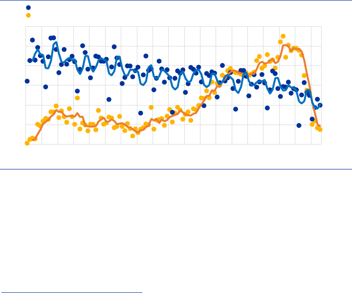
ECB Forum on Central Banking, November 2020
52
GDP, with a subsequent very rapid V-shaped recovery. What explains that quick
recovery?
The answer is found in a series of studies that have documented that the bulk of the
“Trade Collapse” was at the intensive rather than the extensive margin. This is
illustrated in Chart 9, borrowed from Bricongne et al. (2012), which indicates that the
Trade Collapse did not significantly impact the evolution of the number of exporters
in France (which was already on a mild downward trend), while the total volume
exports fell quite dramatically during this period, following more than four years of
steady growth. Overall, Bricogne et al. (2012) conclude that the extensive margin
accounted for slightly over 20% of the trade collapse, a result that they ascribe to the
fact that export entry costs “had already been incurred”. Behrens et al. (2014) found
even starker results for Belgium, where more than 97% of the adjustment for both
exports and imports was at the intensive margin, while Hadad et al. (2010) also
document very muted responses of the extensive margin when using product-level
(not firm-level) information on imports by Brazil, the European Union, Indonesia, and
the United States.
18
One might worry that these patterns were driven by the special
nature of the Global Financial Crisis, but the findings of Bernard et al. (2009) suggest
the external validity of these findings, as they document similar patterns in U.S.
exports to and U.S. imports from several Asian countries during the 1997 Asian
Financial Crisis.
Chart 9
The extensive margin of trade during the great recession
Sources: Bricongne et al. (2012, Figure 1).
In sum, the stickiness of the extensive margin of trade was instrumental in permitting
a swift recovery from the Trade Collapse. Once the crisis subsided, exporters and
importers did not need to incur the large investments that would have been required
to reinstate any broken links, so activity could quickly pick up.
Although these findings suggest that global value chains are remarkably resilient to
shocks, an important caveat with these studies is that they do not focus on the
18
De Lucio et al. (2011), Muraközy (2012) and Jing (2013) provide analogous firm-level evidence for
Spain, Hungary and China, respectively.
40,000
42,000
44,000
46,000
48,000
50,000
52,000
54,000
56,000
58,000
60,000
25,000
27,000
29,000
31,000
33,000
35,000
37,000
01/00
07/00
01/01
07/01
01/02
07/02
01/03
07/03
01/04
07/04
01/05
07/05
01/06
07/06
01/07
07/07
01/08
07/08
01/09
Number of firms (right-hand scale)
Total export: milions (left-hand scale)
ECB Forum on Central Banking, November 2020
53
resiliency of firm-to-firm transactions. In that respect, a more relevant contribution is
the work of Huneeus (2018), who studied firm-to-firm links in Chile and finds a very
small response of these links to small shocks, but a larger response to larger shocks.
Despite the fact that large shocks have the potential to lead to significant
reorganizations of production, the evidence from the Asian Financial Crisis and the
Trade Collapse indicates that even very sizeable global shocks have been
associated with very fast recoveries. The preliminary evidence I will present in
section 7 related to the COVID-19 crisis is consistent with this conclusion.
5 De-globalisation, cost convergence and other long-term
factors
Having discussed technological factors in the last section, I now turn to studying
other long-term factors that may contribute to a future stagnation of globalisation. I
will begin by reviewing the often-mentioned convergence hypothesis, indicating that
higher wage growth in less developed economies relative to advanced economies
has eroded the competitiveness of the former set of countries as hosts of GVC
activity. Competitiveness, however, is a function of productivity as much as of factor
costs, so in section 5.2 I will turn to discussing technology diffusion and how it may
impact globalisation. Finally, in section 5.3 I will analyse other long-run factors
related to structural transformation.
5.1 Wage convergence
As explained in section 3.3, the transition of many countries from inward-looking
socialism or outright communism to market capitalism constituted a massive labour
supply shock from the point of view of firms in advanced countries, as a large pool of
a low-paid, skilled-labour force became available for these firms to hire. At some
level, it is evident that this shock was unique and will not be repeated any time soon.
Although there are certainly many countries in the world that are still not fully
integrated into GVCs, they do not account for as large a share of world population as
the countries listed in Table 1 and, more importantly, they are not as skilled-labour-
abundant as the countries on that list are.
At the same time, the increased labour demand sustained over a period of thirty
years has gradually put upward pressure on the wages of countries that are
recipients of GVC activity, thus naturally eroding the competitiveness of many of
these economies. This is visible in Chart 10, where we see that unit labour costs in
manufacturing have grown much faster in China than in other countries, despite the
marked increase in labour productivity experienced by that country since 1990. More
specifically, the figure plots an index of unit labour costs expressed in U.S. dollars for
China, Germany, Mexico and the United States. The index demonstrates that, since
1990, Chinese unit labour costs have grown about 2.5 times as fast as those in
Germany and the United States. Conversely, the figure shows that despite being
host to a significant amount of GVC activity, Mexican unit labour costs have not
ECB Forum on Central Banking, November 2020
54
grown significantly faster than in the United States or Germany. As a result, many
manufacturing processes continue to be much cheaper to undertake in Mexico than
in the U.S.
Mexico is, however, largely an exception. Many developing countries have
experienced wage pressures similar to those in China, and thus there is now a lower
incentive to move simple manufacturing production processes offshore than there
was in the late 1980s and 1990s. Likewise, there is now a higher incentive to reshore
processes that are no longer performed at significantly lower cost abroad. Will cost
convergence then lead to de-globalisation? It is evident that it will be a contributing
force but, as highlighted in section 4.3, there is a natural asymmetric response of
firms to relative costs shocks depending on whether they are already engaged in
GVC activity or whether they have never offshored before. More specifically, in the
presence of the sunk cost of offshoring, the latter type of firms will need to perceive
large and persistent losses of competitiveness to decide to reshore. In other words,
even if relative costs shocks (perhaps due to exchange rate movements) appear to
make production in a particular location unprofitable, it is not obvious that firms in
advanced economies will want to relocate production right away. Instead, only when
relative cost trends are viewed to be secular trends will firms give serious thought to
abandoning locations that have become prohibitively expensive.
Chart 10
Unit labour cost index in U.S. Dollars (1990=100)
Sources: The Conference Board International Labour Comparisons Program (link).
Importantly, even when firms decide to abandon production in certain countries that
have lost comparative advantage in the processes firms used to undertake there,
this does not necessarily imply that these processes will be reshored to these firms’
domestic economies. This is exemplified by the fact that a significant amount of GVC
activity that used to be carried out in China has already migrated to lower-wage
countries in South East Asia.
Finally, it is also worth remembering that the bulk of multinational firm activity takes
place between countries with similar relative factor endowments and factor prices.
The common consensus a few years ago was that this reflected the dominance of
market-seeking (or horizontal) FDI in overall multinational activity (see Carr et al.,
75
100
125
150
175
200
225
250
275
300
1990 1992 1994 1996 1998 2000 2002 2004 2006 2008 2010 2012 2014 2016 2018
China
Germany
United States
Mexico

ECB Forum on Central Banking, November 2020
55
2001; Blonigen et al., 2003). Nevertheless, work by Alfaro and Charlton (2009)
challenged this view and demonstrated that most FDI flows between advanced
economies have a vertical (input-output) dimension to them. At some level, this
should not be too surprising. The gains from specialization do not rely solely on
factor price differences across countries, but can also stem from idiosyncratic cross-
country differences in productivity in different goods, as the classical Ricardian model
of trade beautifully illustrates. In that sense, the possibility of fragmenting production
across borders gives rise to a finer international division of labour and greater gains
from specialization: GVCs allow resources to flow to their most productive use, not
only across countries and sectors, but also within sectors across stages of
production. A suitable example of the prevalence of fragmentation of production
between relatively similar countries is Boeing’s global production of the 787, which
entails 70 percent of its parts being sourced from 50 suppliers located in 8 developed
economies other than the United States (Japan, Italy, South Korea, France, Sweden,
Canada, United Kingdom and Australia). To sum up, there are good reasons to
believe that convergence in factor prices and in production costs across countries
may not necessarily translate into a de-gobalisation of the world economy.
5.2 Technology transfer
Despite the growth in manufacturing unit labour costs in China, Chinese labour
productivity has increased dramatically since 1990.
19
This has allowed firms in the
West to continue to find that country a suitable location of production for many
industrial processes. Yet Chinese technological absorption has also generated a fair
amount of anxiety in advanced economies, as is exemplified by President’s Trump’s
frontal opposition to China’s quid pro quo policy – a policy that makes technology
transfer a precondition for foreign firms to be able to operate in China. I will offer
some brief thoughts below on the specifics of the U.S.–China technology war, but I
will first consider more broadly the effects that technology transfer may have on the
future of globalisation.
Should advanced economies fear the technological advance of less developed
economies? Will it undermine the future of globalisation? Although focused on
somewhat distinct aspects, these two questions are at least partly intertwined. To
see this, and relying on the classical analysis of technology transfer in neoclassical
trade theory (see Johnson, 1955), it is well known that technological improvements
in foreign countries are typically beneficial for a specific country. The only exception
is whenever foreign countries improve upon technologies related to goods for which
that specific country had a comparative advantage before the technological catch-up.
The reason for this is that in those situations, productivity growth abroad worsens a
specific country’s terms of trade. The flip side of this effect is that such a form of
technology transfer erodes the gains from specialisation and reduces gross trade
19
The same Conference Board International Labour Comparisons Program data used in Chart 10
indicates that real value added per employed person was almost 14 times larger in 2018 than in 1990
(link).

ECB Forum on Central Banking, November 2020
56
flows across countries. In sum, technological change abroad is detrimental to
advanced countries precisely when it leads to de-globalisation.
The mid 2000s witnessed a heated debate – involving the almost nonagenarian Paul
Samuelson and Jagdish Bhagwati and co-authors – concerning the extent to which
offshoring by U.S. companies had fuelled export-biased technological change by
less-developed economies. Samuelson (2004) argued that this was a theoretical
possibility and offered a carefully chosen numerical example in which offshoring-
induced productivity growth in China completely kills off trade between the U.S. and
China! Bhagwati et al. (2004) admitted the theoretical argument, but argued that the
phenomenon of offshoring should be better thought as one in which processes that
in the past had not been able to be sliced across countries suddenly became
tradable, thereby improving welfare worldwide. As stimulating as this debate was,
and as pointed out by Dixit and Grossman (2005), there was no evidence that the
U.S. terms of trade had deteriorated significantly, so the debate faded as quickly as it
had flared up.
Anxiety over technological advancement in China has erupted again in recent years,
with many governments in advanced economies demanding that China take a
tougher stance on intellectual property rights (IPR) protection. President Trump has
been particularly forceful about this, criticizing the Chinese quid pro quo policy and
specifically targeting certain Chinese companies (such as Huawei, WeChat or
TikTok) with specific restrictions or bans. What is the likely effect of these demands
on stronger IPR protection? Will they lead to more reshoring and contribute to a de-
globalized world?
In order to answer this question, it is worth pausing to carefully delineate the precise
role for government intervention in this particular situation.
20
When an American firm
willingly forms a joint venture with a Chinese firm, what externality is the U.S.
company not internalizing? Presumably the company understands that because IPR
protection in China is not as strong as in the United States, that joint venture
increases their risk of the technologies they share with their Chinese counterpart
being leaked to other producers in China. If the firm correctly anticipates the
probability of leakage, and I see no reason to believe why it would not, then it would
internalize the loss in the net presented discounted value of its future profits
associated with the higher probability of technological theft. Still, the cost advantage
or market-access benefits associated with joint ventures in China lead some U.S.
firms to find it optimal to operate there, though they might do so without sharing their
state-of-the art technologies.
Against this backdrop, if the ongoing spat between China and other advanced
economies results in China putting in place stronger IPR protection laws, it is very far
from obvious that this will trigger a process of reshoring. On the contrary, such
20
I focus here on the role of technological spillovers, but governments may still play a useful role in the
absence of such externalities. For instance, if the “quid pro quo” policy is viewed as a “tax” on U.S.
multinationals operating in China, and if the U.S. government is in a better position than U.S. firms to
convince the Chinese government to reduce or eliminate that tax, then such government pressures
might be beneficial.

ECB Forum on Central Banking, November 2020
57
stronger IPR protection might provide incentives for new firms to slice their value
chains and operate in China, especially for firms that are unwilling to share their
technologies in a joint venture in the current environment. Indeed, this is in line with
the findings of the literature on the effects of the tightening of IPR protection on U.S.
multinationals’ operations. In particular, Branstetter et al. (2006) and Bilir (2014)
found that patent law reforms that improved IPR protection abroad are associated
with U.S. multinationals transferring more technology to their foreign affiliates, with
the effects being disproportionate in sectors with long product life cycles. In sum,
although the current tensions between the U.S. and China have fuelled concerns
about de-globalisation, it is far less obvious that the “U.S.–China technology war” will
be hugely detrimental to U.S. multinational activity in China.
21
Let me conclude this section by stressing that my thoughts above on the
technological wars have focused on positive rather than normative aspects. Even if
one concedes that investments by U.S. firms in China are privately optimal, it is far
less obvious that they will be socially optimal. In particular, firms may not internalize
the effects that their technological leakage might have on other U.S. firms, or on the
U.S. more broadly, as has been highlighted by commentators that have warned
about the cybersecurity issues associated with global value chains.
5.3 Structural transformation, investment and capital goods
In this section, I briefly touch upon additional long-term forces that may potentially
contribute to a process of de-globalisation.
First, consider the role of structural transformation, which involves a secular shift of
economic activity from manufacturing to services, much like the structural
transformation that turned agrarian economies into industrialized ones. Because
manufacturing goods are more easily tradable than many services, it would appear
that as a higher percentage of world GDP is accounted for by services, the ratio of
world trade to world GDP will necessarily face downward pressure, thus confirming
fears of de-globalisation. This argument, however, holds the relative tradability of
manufacturing and services to be constant over time, while I have argued in section
4.2 that new technologies have and will continue to enhance the ability of economic
agents to trade services at long distances. Indeed, consistent with the
counterbalancing effects of these two forces, panel A of Chart 11 demonstrates that
the ratio of service exports to GDP has grown much faster (from 4% in 1995 to
almost 7% in 2018) than the ratio of overall services to GDP (which grew from 55%
to 65% in the same period).
21
A telling illustration of this claim is the decision by Tesla to begin assembling their electric cars in China
once the company was assured that it could maintain whole ownership of their factories in that country.

ECB Forum on Central Banking, November 2020
58
Chart 11
Structural transformation and composition effects
Sources: World Development Indicators.
A second secular trend is associated with the notion that the pattern of economic
growth across countries has changed since the Great Recession, and relatively open
economies now grow slower than relatively more closed economies. If this were a
fact, world openness would be expected to be on a downward trend, as economies
that are relatively more closed capture a larger and larger share of world trade.
Nevertheless, as panel B of Chart 11 indicates, there is virtually no correlation
between the cross-section of GDP growth rates in the period 2009-2018 and the
cross-section of exports to GDP ratios in 2007.
22
In words, it does not seem that the
premise for this mechanism holds in the data.
22
The relationship is mildly negative and turns a bit more negative when dropping countries with export
shares higher than 1. But as soon as one weights the observations by GDP or population in 2007, the
relationship turns mildly positive (though insignificant).
3%
4%
5%
6%
7%
30%
35%
40%
45%
50%
55%
60%
65%
70%
1995 1997 1999 2001 2003 2005 2007 2009 2011 2013 2015 2017
Services/GDP (left axis)
Service Exports /GDP (right axis)
a) Exports over GDP vs. Service Exports over GDP
-4%
-2%
0%
2%
4%
6%
8%
10%
0 0.5 1 1.5 2 2.5
GDP Growth (2009-2018)
Exports over GDP
b) Openness and GDP Growth (2009-18)
ECB Forum on Central Banking, November 2020
59
Chart 12
The decline in investment rates
Sources: García-Santana et al. (2020). World Investment Indicators (link).
Notes: For panel A, data have been all been filtered out from country fixed effects. Projections (in red) based on a cubic polynomial of
log GDP per capita.
The last secular force I will elaborate on is more intriguing and relates to the marked
decline in investment rates in many countries in recent years. It has been a matter of
debate whether this decline will be a permanent one or transitory, but panel A of
Chart 12, borrowed from García-Santana et al. (2020), indicates that the relationship
between country-level investment rates and the level of development (measured by
log GDP per capita) exhibits a clear inverted-U shape in the data for the period 1950-
2011. Furthermore, aggregate world GDP per capita currently features a value well in
excess of $7,125, which corresponds to the value of GDP at which investment rates
peak according to the cubic fit in the figure. Indeed, as panel B of Chart 12 shows,
the aggregate world investment rate has been on a clear downward trend in the last
50 years. This phenomenon is particularly relevant for world trade because
investment goods (capital goods, machinery, transport equipment, etc.) constitute
about forty percent of merchandise trade. A secular slump in investment is thus likely
0.0
0.1
0.2
0.3
0.4
0.5
6.5 7 7.5 8 8.5 9 9.5 10 10.5 11 11.5
log GDP per capita
a) World Investment Rate (World Gross Capital Formation as % of World GDP)
0.22
0.23
0.24
0.25
0.26
0.27
0.28
0.29
1970 1973 1976 1979 1982 1985 1988 1991 1994 1997 2000 2003 2006 2009 2012 2015 2018
b) Investment Rate and Level of Development (By country and year, 1950-2011)

ECB Forum on Central Banking, November 2020
60
to reduce the share of world trade flows in the overall level of economic activity in the
world.
23
6 De-globalisation and policy factors
In section 4, I fleshed out a series of arguments questioning the view that
technological factors (such as automation) are likely to constitute a secular force
fostering a retreat in globalisation in the coming decades, while in section 5 I have
studied the plausibility of additional secular non-policy drivers of de-globalisation. In
this section, I will instead focus on the role of policy factors in potentially leading to
an era of increased isolationism, much as occurred in the 20th-century Interwar
Period.
It is intuitively clear that the policy and institutional factors that fuelled the era of
hyperglobalisation are much more reversable than the technological ones. Although
it is hard to imagine that Eastern Europe will again fall behind an iron curtain or that
China will abandon market economy practices, trade policies (and economic policies
more broadly) can easily turn much more protectionist than they have been in the
recent past. In principle, multilateral and regional trade agreements were designed in
ways that mean they cannot easily be reversed, but recent events have undoubtedly
eroded the notion that freer trade is necessarily here to stay. How likely is it that the
next few years will bring a policy- or institutionally-driven process of de-globalisation?
The rest of this section will provide tentative answers to this question.
6.1 Stalling liberalization and burgeoning protectionism
Scepticism about the sustainability of the liberalized environment that was so
conducive to the growth of global value chains is justified by at least three types of
recent developments.
First, it is evident that the multilateral liberalization agenda under the umbrella of the
WTO is at an impasse. The current round of negotiations, the Doha round, began in
November 2001, and has yet to reach a conclusive agreement. Admittedly, the round
began with an already very low average level of protection (see Chart 8), and it
attempted to tackle very sensitive issues, such as the removal of agricultural
subsidies in the U.S. and the European Union. Yet, the lack of substantial progress in
close to twenty years has led many countries to lose faith in the ability of the WTO to
further push the liberalization agenda.
23
A lingering question is: will investment rates continue to fall permanently in the future? Given available
estimates of the elasticity of substitution between capital and labour, the transitional dynamics of the
“good old” neoclassical growth model indeed predict that investment rates will feature the inverted-U
pattern in panel C of Chart 11 (see Antràs, 2001, 2004). The recent revival of the admittedly much
sexier secular stagnation hypothesis (see Summers, 2011) also predicts a secular decline in
investment for years to come.
ECB Forum on Central Banking, November 2020
61
Second, the process of regional liberalization has also largely stalled and, more
worryingly, it shows signs of being in retreat. The decision of the United Kingdom to
leave the EU, voted for in the referendum in June of 2016 and ratified in January of
2020, is an evident example of this trend. At the time of writing, it is not entirely clear
what the implications of Brexit will be for the ease of flow of goods and services
between the UK and the other members of the EU, but it is undoubtedly clear that
Brexit will reduce their economic interdependence. Another example is President
Trump’s insistence on renegotiating NAFTA, culminating in the signing of the United
States-Mexico-Canada Agreement (or USMCA, for readers inclined to pronounce
institutions by their acronyms – good luck with this one!). Much has been written
about the provisions in the new agreement regarding rules of origin in the automobile
industry and labour standards in Mexico, but a particularly worrisome aspect of this
agreement is the so-called “sunset clause,” which stipulates that the agreement must
be reviewed by the three nations every six years, and that it will expire after sixteen
years unless it is unanimously decided to extend it. Naturally, this makes future trade
integration between the U.S., Canada and Mexico much more uncertain than it was
under NAFTA. Even before the election of President Trump in 2016, appetite for the
signing of the Transatlantic Trade and Investment Partnership (TTIP) and the Trans-
Pacific Partnership (TPP) had largely waned in the United States, as exemplified by
the fact that the Democratic candidate, Hillary Clinton, did not support the signing of
these agreements either. Relatedly, free trade agreements have become more
difficult to negotiate due to the many additional provisions that have become part and
parcel of such agreements: in the lingo of trade economists, we live in the age of
“deep” rather than “shallow” trade agreements.
Chart 13
Average U.S. tariffs in the Trump age
Sources: Amiti, Redding and Weinstein (2019, Figure 3).
A third, much more worrisome development is the recent U.S.–China trade war.
Starting in early 2018, President Trump enacted a series of tariff increases on
specific products and countries, with China as an explicit target. Import tariffs
increased from 2.6% to 16.6% on 12,043 products covering $303 billion (12.7%) of
annual U.S. imports (see Fajgelbaum et al., 2020). As a result, and as Chart 13
shows, average (weighted) U.S. tariffs more than doubled in 2018. In response to
these unilateral measures, U.S. trade partners (and China, in particular) imposed
0
1
2
3
4
5
6
12/17
01/18
02/18
03/18
04/18
05/18
06/18
07/18
08/18
09/18
10/18
11/18
12/18
01/19
02/19
03/19
04/19
05/19
06/19
07/19
08/19
09/19
10/19
11/19
Solar and
Washing
Machines
($10B)
Steel and
Alum.
($18B)
Steel and
Alum.:
Canada,
Mexico,
EU ($22B)
China 1
($34B)
China 2
($16B)
China 3
($200B)
Increase on
China 3
($200B)
China 4
($112B)
Percent
ECB Forum on Central Banking, November 2020
62
retaliatory tariffs on U.S. exports. Beyond the increases in average tariffs associated
with these developments, there is a growing sense that the WTO is too weak an
institution to restore order to the current situation.
6.2 Underlying forces
What triggered the recent political backlash against globalisation? Answering this
question is particularly important if one wants to understand the extent to which the
forces that led to this escalating protectionism are only temporary or are instead
secular.
A first obvious but important point is that recent protectionist spats have not been
triggered by idiosyncratic decisions of particular individuals or political parties. Nigel
Farage might have played a singular role in Brexit, and President Trump’s blunt
approach to policy making might have precipitated the U.S.–China trade war. But
these individuals, as well as many other champions of protectionism around the
globe (such as Bolsonaro in Brazil or Orban in Hungary) are elected officials who
reached powerful positions because their electoral platforms appealed to a broad
share of their electorates.
Consistent with this, data from surveys of people’s perception of the consequences
of trade for their economies suggests that the last few years of the hyper-
globalisation period witnessed a significant share of people voicing concerns about
the consequences of trade integration. Chart 14 provides an illustration based on the
perceived effects of foreign trade in the United States. More specifically, Gallup has
been asking Americans for close to thirty years the question: “What do you think
foreign trade means for America? Do you see foreign trade more as an opportunity
for economic growth through increased U.S. exports or a threat to the economy from
foreign imports?” As the left panel of Chart 14 shows, in the early 2000s the share of
people responding that trade was good for the economy declined from 56% in 2000
to 41% in 2008, with the flip side of this being an increase in the share of people
viewing trade as an economic threat increasing from 35% in 2000 to 52% in 2008.
The increasing discontent with globalisation was widespread along the political
spectrum. As the right panel of Chart 11 shows, support for globalisation fell
dramatically in 2000-08 for both Republican as well as Democratic voters.
Given the patterns in Chart 14, it is not entirely surprising that the 2010s witnessed a
proliferation of politicians and political parties catering to these increased demands
for protectionism. Ironically, Chart 14 also demonstrates that perceptions of the
consequences of trade for the U.S. economy have changed dramatically since 2008,
and last year, prior to the COVID-19 crisis, 74% of respondents revealed seeing
trade in a positive light, and only 21% characterized it as a threat. The recent trend
might reflect improving economic conditions up to the COVID-19 shock, but Gallup
also found that many more respondents (45%) indicated that the U.S.–China trade
war was harmful to the economy rather than beneficial (31%), despite the fact that
62% described China as engaging in unfair trade practices.
ECB Forum on Central Banking, November 2020
63
Although support for protectionism might be much lower today than it was in the
aftermath of the Great Recession, it is worth analysing the underlying causes of the
growing discontent in the early 2000s, so as to better understand whether this
discontent is likely to continue to wane in coming years or whether it may instead
reinflame.
Chart 11
Perceived effects of foreign trade in the United States
Sources: Gallup (2019, Figure 1, link).
As many commentators have pointed out (see Pavcnik, 2017, Rodrik, 2020), a key
source of resentment is related to the distributional effects of international trade.
During the hyperglobalisation period, not only did economies become much more
interconnected, but many of these economies contemporaneously experienced a
significant rise in income inequality. For instance, during 1979-2007, the Gini
coefficient associated with the distribution of U.S. market income grew dramatically
from a level of 0.48 all the way to 0.59. Furthermore, as is clear from the left panel of
Chart 15, trade integration and inequality grew very much in parallel even at fairly
high frequencies. The extent to which these two phenomena are causally related has
been the subject of intense academic debate, but it is by now a widely accepted view
that trade integration has been a nonnegligible contributor to increased income
inequality in the U.S., in many other industrialized countries, and even in developing
20%
30%
40%
50%
60%
70%
80%
1992 1994 2000 2001 2002 2003 2005 2006 2008 2009 2011 2012 2013 2014 2015 2016 2017 2018 2019
Opportunity for the economics growth
Threat to the economy
a) Overall Population
20%
30%
40%
50%
60%
70%
80%
1992 1994 2000 2001 2002 2003 2005 2006 2008 2009 2011 2012 2013 2014 2015 2016 2017 2018 2019
Democrats
Republicans
b) Trade is Good by Political Affiliation

ECB Forum on Central Banking, November 2020
64
countries (see Krugman, 2008, Goldberg and Pavcnik, 2007). A couple of landmark
academic papers in the 2010s – Autor, Dorn and Hanson (2013) and Pierce and
Schott (2016) – further singled out trade integration with China as a particularly
salient contributor to the decline in U.S. manufacturing employment in the 1990s and
2000s.
Trade-induced increases in inequality need not generate discontent as long as those
that may be harmed by trade integration are properly compensated. Have the losers
from globalisation been compensated? In Antràs, de Gortari and Itskhoki (2017), we
estimate the average degree of tax progressivity in the United States tax-transfer
system and found a very significant decline in the degree of tax progressivity over
the same period 1979-2007 in which the U.S. economy became much more
integrated in world markets and was experiencing a marked increase in inequality in
the distribution of market (pre-tax) income (see panel B of Chart 15).
24
In sum, in a
period during which import competition was putting significant pressure on real
wages and employment, the U.S. safety net was being pulled out from under U.S.
workers’ feet. Because median real weekly earnings grew very meagrely in the
1980s, 1990s and 2000s (see Acemoglu and Autor, 2011), it is natural that a growing
share of U.S. workers felt alienated by the process of globalisation, despite the fact
that aggregate real income in the U.S. grew significantly during this period.
25
24
To compute this index of tax progressivity, we used information on the distribution of adjusted gross
income in public samples of U.S. IRS tax returns, as well as CBO information on the tax liabilities and
transfers received by households at different points of the U.S. income distribution.
25
Even from a utilitarian social welfare perspective, the welfare gains associated with international trade
would be about 20% lower than those implied by aggregate real income (see Antràs, de Gortari and
Itskhoki, 2017).
ECB Forum on Central Banking, November 2020
65
Chart 15
Inequality and redistribution in the United States
Sources: Antràs, de Gortari and Itskhoki (2017).
Although globalisation might have created some discontent, it is less clear the extent
to which trade-induced inequality directly contributed to the emergence of the
protectionist and isolationist policies we have seen put in place in the last few years.
Recent literature, both theoretical as well as empirical, has studied such a link. On
the theoretical side, Grossman and Helpman (forthcoming) borrow tools and insights
from social psychology to argue that increased income inequality may generate
endogenous changes in social identity that generate a protectionist bias in trade
policy. On the empirical front, Autor et al. (2020) and Colantone and Stanig (2018a)
establish a causal link between the China (import competition) shock and (i) a rise of
political polarization in the U.S. and (ii) an increase in support for nationalist and
isolationist parties in 15 Western European countries, respectively. A couple of
spinoffs of these papers – Autor et al. (2017) and Colantone and Stanig (2018b) –
have further directly linked the China shock to the outcomes of the 2016 U.S.
presidential election and the 2016 Brexit referendum vote, respectively.
0.5
0.5
0.5
0.5
0.6
0.6
0.6
4%
5%
6%
7%
8%
1979 1983 1987 1991 1995 1999 2003 2007
Gini of Market Income (right axis)
Trade/Gross Output (left axis)
a) U.S. Trade Openness and Gini Coefficient
0.1
0.1
0.2
0.2
0.2
0.3
1979 1983 1987 1991 1995 1999 2003 2007
Tax Progressivity Index
b) Index of U.S. Tax Progressivity

ECB Forum on Central Banking, November 2020
66
6.3 Implications for the future of globalisation
With this background in mind, we are now ready to revisit the main theme of this
paper, which concerns the future of globalisation. What would the consequences be
of persistent trade wars across countries? Are the forces that fuelled the backlash
against globalisation in the early 2000s likely to re-emerge in coming years and
indeed make policy spats persistent? And might the ongoing COVID-19 health crisis
spark an intensification of the resentment against globalisation? I will postpone
tackling the last question until section 7, which will focus on the current global
pandemic, but we can attempt to isolate an answer to the first two questions by
(hypothetically) rolling back time to January of 2020.
Let me first discuss how the persistence of trade wars would impact the future of
globalisation. The answer here is fairly clear, as the Interwar Period reminds us, but
it is worth commenting on a few nuances.
First, it is not immaterial whether trade wars continue to be bilateral in nature, as is
largely the case with the current U.S.–China trade, or whether the situation escalates
into an all-out world trade war. In the former case, and as some studies have already
shown (see Flaaen et al., 2020), production might relocate to (third) countries
unaffected by the bilateral trade war rather than being reshored to domestic
economies. If tensions turn multilateral in nature, however, a scenario of significant
de-globalisation would become much more likely.
26
Second, because of the relevance of sunk costs, the perceived persistence of trade
disputes will be key for the extent to which production will relocate across countries.
In this sense, the outcome of the November 3rd presidential election in the U.S. is
encouraging and suggests a decrease in policy isolationism in the U.S. (although,
frankly, the stance of the future Biden administration on U.S. trade relationships with
China remains somewhat unclear). Nevertheless, to the extent that continuing
pressures for nationalist trade policies lead to the weakening or potential
disbandment of the WTO, we could well face a very serious threat to the architecture
that underpinned the process of trade liberalization in the post-WWII era.
A third relevant factor is that recent developments have not only increased the
average level of tariffs but have also generated a lot of trade policy uncertainty. Such
uncertainty is likely to weigh on the decision of firms to make new investments in
China, and might also lead some firms to diversify their sourcing strategies (possibly
involving partial reshoring) in situations in which they are able to afford the fixed
costs associated with more complex, multi-sourcing strategies.
Finally, it is worth mentioning an additional potential ramification of the current Sino-
American trade tensions. As some commentators have pointed out, there is the real
risk that geopolitical and strategic imperatives drive a decoupling and a
26
Empirical work on the economic impact of the U.S.-China trade war is still at its infancy, but a slowly
emerging body of work seems to indicate that the increased trade barriers in Chart 13 and the
retaliation they triggered from China, has harmed both U.S. consumers (see Amiti et al., 2019,
Fajgelbaum et al., 2020) and also the U.S. manufacturing sector (see Flaaen et al., 2020, Handley et
al., 2020).
ECB Forum on Central Banking, November 2020
67
fragmentation of the world economy into hostile political blocs, with a potential
bifurcation of technology standards that would undermine much of the digital
integration achieved in recent decades. A world partitioned into two “internets”, a
Western one and a Chinese one, where the latter would only allow users and apps
that sign up to China’s regulatory and compliance standards would pose a serious
threat to the process of global integration.
Having outlined the consequences of persistent trade tensions, I next turn to the
arguably more fundamental second question of whether the backlash-generating
forces discussed in section 5.2 are likely to persist in the next few years. From the
vantage point of January 2020, the key consideration for answering this question
was: will we continue to see trade-induced inequality in the coming years, and will
redistribution systems continue to insufficiently compensate the losers from
globalisation? In this respect, it is honestly hard to be optimistic. I have argued in
section 4.2 that recent technological developments (such as automation and the
proliferation of digital platforms) might well give globalisation a second wind, but it
also seems likely that these technological developments will aggravate income
inequality in both advanced and less developed economies. Consider the case of
automation. Although I have argued that industrial robots, 3D printing and other
automated forms of production might well lead to the growth in trade in
complementary inputs of production, it is also evident (and has been empirically
established) that they tend to reduce the demand for workers (and particularly
production workers) in advanced economies (see Acemoglu and Restrepo, 2020,
Acemoglu et al., 2020). Furthermore, while automation might have a positive effect
on offshoring in less developed economies (as documented by Artuc et al., 2018, or
Stapleton and Webb, 2020), it is likely that the increased demand for foreign labour
will be biased in favour of skilled workers in those less developed economies, in line
with the vast literature documenting the skilled-labour intensity of GVC activity (e.g.,
Verhoogen, 2008). In sum, automation is likely to increase inequality both by
reducing the labour share of income, and also by giving a higher share of that labour
income to relatively skilled workers worldwide.
In the case of digital platforms, despite their enormous potential to enhance the
efficiency of international trade in consumer goods and intermediate inputs, the
same reputation mechanisms GVCs rely on to verify seller and buyer quality may
foster concentration, thus making it harder for entrants to compete. Within existing
firm-to-firm GVC links, novel technologies might also have implications for the
relative bargaining power of the different participants in GVCs. For instance, digital
platforms might allow large buyers in rich countries to gain information on a larger
number of potential suppliers, thus enhancing their ability to have these suppliers
compete with each other. This in turn may lead to better terms of trade for lead firms
in rich countries, at the expense of a lower share of the gains from GVCs accruing to
producers in less developed economies. Furthermore, digital platforms themselves
have been accumulating vast amounts of information on the users of their platforms,
and this certainly enhances their ability to use this information to their advantage,
either by locking in buyers with particularly well-tailored recommendations, or by
price discriminating in particularly effective ways. As a result, digital platform firms
ECB Forum on Central Banking, November 2020
68
also pose new challenges for regulators seeking to ensure fair competition and
prevent abuses of market power.
Concerns about growing market power of firms engaged in GVC activity are
compounded by the widespread profit-shifting practices of these companies, which
have found it relatively simple to exploit loopholes in international taxation laws to
increase the share of their profits that are accrued in locations with particularly low
(or even zero) corporate tax rates.
The inability of regulators to adequately tackle the issue of profit-shifting also
resonates with the inability (or unwillingness) of many governments to put in place
sufficiently progressive tax systems to ensure that the gains from economic growth
and international trade are widely spread in the population. Although discontent over
globalisation and inequality has given rise to populist governments in many parts of
the globe, in most cases those governments have been right-wing rather than left-
wing so if anything they have been less inclined to increase the progressivity of their
tax systems (see Rodrik, 2020).
Despite these pessimist views, remember that recent Gallup surveys show a marked
increase in support for globalisation since 2008, at least in the U.S. This indicates
that views on globalisation are strongly correlated with economic cycles, regardless
of how widely spread the benefits of economic growth are. As puzzling as this may
be, it suggests that as long as the world avoids long recessions, we may also avoid
de-globalisation.
Now, in the last few paragraphs I had hypothetically turned back time to January of
2020, but it is now time to tackle the big elephant in the room.
7 The COVID-19 crisis and the future of GVCs
I conclude this paper with a discussion of how its main themes interlace with the
global pandemic the world is actively fighting at the time of writing. What has been
the immediate impact of the COVID-19 pandemic on global integration and GVC
activity more narrowly? What are the likely mid- to long-run implications of this crisis
for the future of globalisation and of GVCs? Although answering these questions
satisfactorily would require an essay of its own, and could also benefit from a few
more months (or even years) of enhanced perspective, I will attempt to provide some
tentative answers below, appealing to the insights offered earlier in this paper.
7.1 The COVID-19 health crisis
The background of the COVID-19 (or Coronavirus) global pandemic is well known by
now. The epidemic originated in Wuhan, China, where the first cases were identified
in December of 2019. By January 2020 there was a widespread awareness that this
was a serious epidemic with the potential to turn into a global pandemic. Indeed, on
January 21, 2020, the first human-to-human infections of COVID-19 in Europe are
ECB Forum on Central Banking, November 2020
69
presumed to have taken place in Starnberg, Germany, when a local car parts
supplier (Webasto) organized a training session with a Chinese colleague from its
operation in Wuhan. The epidemic grew quickly in Europe during February and
March of this year, with a particularly heavy death toll in Italy and Spain. The first few
cases in the United States were diagnosed in late January, but the disease only
became an epidemic in March. A well-known focus of infection was a biotech
conference in Boston, Massachusetts, on February 22-23, 2020, which is believed to
have spread the disease to at least six states in the U.S. and three European
countries, and caused close to 100 infections in Massachusetts alone. By March
11th, 2020, the epidemic had spread to essentially all corners of the world, and the
World Health Organisation declared COVID-19 a global pandemic. At that point in
time, only around 4,300 people had died worldwide. At the time of writing, early
November of 2020, the death toll of the COVID-19 pandemic had reached 1.3 million
deaths, with no clear end to the epidemic in sight despite gargantuan efforts to
develop an effective vaccine.
As we have emphasized in Antràs, Redding and Rossi-Hansberg (2020),
globalization and pandemics are closely intertwined. Not only was the rapid spread
of the disease an obvious consequence of the globalized nature of economic activity
and of GVC activity more narrowly – as the Starnberg and Boston examples above
illustrate – but the global pandemic has had a severe impact on the workings of the
global economy. Most notably, the flow of people across borders has essentially
come to a halt both due to government restrictions but also due to purposeful social
distancing practices by individuals. But beyond migration flows, the profound and
asynchronous nature of the COVID-19 shock has also had an immediate impact on
world trade flows, as the next section will overview.
7.2 Short-term effects
Although at this point in time the data we have at hand is somewhat tentative in
nature, Chart 16 attempts to provide a preliminary diagnostic of the impact of the
global pandemic on the flow of goods across countries. In panel A I use data from
the CPB (Netherlands Bureau for Economic Policy Analysis) to illustrate the dramatic
decline in world trade in recent months. Relative to its level in August of 2019, world
trade reached the bottom in May of 2020, when it had reached a cumulative decline
of 17.6%. In June, July and August however, trade flows grew at a fast pace, and by
the end of August, the year-on-year decline in trade had been reduced to a much
more moderate 4.4%. The figure shows that although industrial production also
markedly declined during the crisis, the response of world trade has been slightly
larger. It is important to emphasize, however, that the current pandemic is affecting
the service sector much more than the industrial sector, so it is quite likely that by the
end of 2020 the ratio of world trade to world GDP will be significantly higher than it
was at the end of 2019.
Panel B of Chart 16 further decomposes the evolution of world trade during the
current calendar year into different types of goods. The data originates in the creative
work of Cerdeiro et al. (2020), who use data from radio signals emitted by global
ECB Forum on Central Banking, November 2020
70
vessels for navigational safety purposes to construct estimates of world seaborne
trade (in terms of metric tons) based on the dimensions and characteristics of the
ships. The data is available at a very high-frequency (daily) and with a short lag, so
despite its imperfect nature it provides a valuable angle on the recent decline in
trade. A few patterns in the figure are noteworthy. First, the chart illustrates clearly a
“double-dip” in world trade, first in February and then again in April and early May,
reflecting lockdowns (and social distancing) first in China, and then in Europe and
North America. Second, although world trade was 11% lower in early June than in
early January, by early October world trade had fully recovered to its level at the
beginning of the year, thus confirming that world trade is recovering much faster than
world GDP. Third, information on the type of vessel used for transport allows one to
decompose the evolution of world trade into various components associated with
bulk carriers, oil/chemical tankers, general cargo/container ships and vehicle
vessels. The chart then demonstrates that world trade in vehicles, a prototypical
example of GVC trade, experienced a much larger initial decline (at some point a
cumulative decline of 50%) than other types of trade. Nevertheless, this type of trade
also recovered faster than other components of trade, and by early September it had
reached early January levels. Whether the disproportionate rise and fall of vehicles
in panel B reflects the peculiarities of GVC trade or the durable nature of the goods
being shipped is an open question, but in any case the figure demonstrates that
standard indices of globalisation based on trade statistics are not likely to provide
ammunition for those commentators advocating for the advent of an era of de-
globalisation in the near future.

ECB Forum on Central Banking, November 2020
71
Chart 16
The impact of COVID-19 On world trade
Sources: Antràs, de Gortari and Itskhoki (2017).
Why has world merchandise trade recovered so quickly from the May lows?
Unfortunately, the characteristics of the data we have at hand at this point in time are
not conclusive, but the conceptual considerations developed in section 4.3 of this
paper, as well as empirical evidence from the Great Recession and the 1997 Asian
Financial Crisis reviewed in that same section, leads me to hypothesize that the
trade collapse in Chart 16 has not operated, at least up to this point, at the extensive
margin. This conjecture also explains the rapid recovery in world trade from May to
September, and it also suggests that as long as the global pandemic is not perceived
to be a highly persistent shock, the medium-run implications of the current health
crisis for world trade will be muted.
27
On the latter matter, and even if we are still in
the midst of much uncertainty about the timing and effectiveness of a COVID-19
27
This is indeed consistent with the calibration results in Antràs, Redding and Rossi-Hansberg (2020).
Furthermore, preliminary evidence from Spanish Customs data suggest indeed that less than 5% of the
decrease in Spanish exports during March-August of 2020 relative to March-August of 2019 was
explained by the intensive margin (see Minondo, 2020).
80
85
90
95
100
105
07/2019 09/2019 11/2019 01/2020 03/2020 05/2020 07/2020
World trade
World Industrial Production
a) World trade and world industrial production (Index July 2019 = 100)
40
50
60
70
80
90
100
110
120
01/01 01/02 01/03 01/04 01/05 01/06 01/07 01/08 01/09 01/10
Bulk
Container
Oil/chemicals
Total
Vehicles
b) Estimated metric tons of world exports (30-day moving average in ratio to 2017-19 average)
ECB Forum on Central Banking, November 2020
72
vaccine, it seems reasonable that this shock is still widely perceived to be more
transitory than the Great Recession. As a result, it is then natural that firms are at
this point unwilling to sever international ties and reshore activity domestically.
7.3 Medium-to-long-term effects
Even if in the short-to-medium run merchandise trade recovers to pre-COVID-19
levels, it is worth pausing to elucidate whether the current global pandemic might
sow the seeds of an intensified phase of de-globalisation. To answer this question, it
is useful to again separate effects working largely through technology, and effects
working through policy.
On the technological front, there are reasons to believe that the decline in face-to-
face interactions experienced in recent months is likely to persist (though obviously
in a less dramatic manner) for years to come. On the one hand, it is hard to gauge
the state in which the airline industry will leave the crisis, but it seems inevitable that
international travel will be less pleasant and more expensive for years to come. On
the other hand, even with a vaccine in place, the willingness of people to share tight
places, like airplanes, with other individuals is likely to remain depressed for some
time. To the extent that face-to-face interactions and international business travel are
important inputs into the well-functioning of GVCs, it seems reasonable to expect a
reshoring of economic activity in ways that diminish the need for long-distance travel.
Indeed, there is a small but fruitful empirical literature that has demonstrated the role
of international business travel in facilitating international trade (see Cristea, 2011,
Blonigen and Cristea, 2015, and Startz, 2018) and, more generally, in fostering
economic development (see Campante and Yanagizawa-Drott, 2018).
It is pertinent, however, to mention two caveats to this argument. First, the marginal
return to face-to-face interactions is likely to be larger when initiating trade
relationships than when maintaining them, so I would expect the effect of depressed
international business travel on world trade to operate largely at the entry margin
rather than at the exit margin. In plain words, business executives are unlikely to
shut down existing offshore plants due to increased nuisances in international travel,
but they are likely to take these matters into consideration when considering the
location of new plants. As a result, the adjustment might only materialize gradually.
Second, it may perhaps be naïve to ignore the possibility that future technological
developments will enhance virtual interactions in ways that make them much more of
a substitute for face-to-face interactions. Such developments would of course tilt the
balance toward a more globalised world economy (albeit with less international
travel).
These technological considerations are, however, second-order relative to the
impact of the political landscape post COVID-19 on GVCs. Will the current pandemic
add fuel to the fire in the current political tensions between the U.S. and China? Or
will a global coordinated effort to eradicate the global pandemic produce some
goodwill that can then be used to ease tensions in the future? The answer to these
ECB Forum on Central Banking, November 2020
73
questions in part depends on the stance of the future Biden administration in the
United States, but at this point in time I see two main reasons for pessimism.
First, the pandemic has brought about a number of diplomatic disputes related to the
exact origin of the COVID-19 crisis, with President Trump making a concerted effort
to publicly refer to it as the “Wuhan virus” or the “China virus.” Tensions have also
flared up in Europe, where the passing of a massive aid package was delayed until
late July and only after many heated rounds of negotiations and mutual
recriminations. These types of finger pointing and blame games are not likely to be
conducive to healthy international relations in the future, and they do not bode well
for the future of global organizations such as the WTO (which incidentally has been
without an interim Director-General for more than two months at the time of writing).
A second reason for concern relates to the highly regressive nature of the economic
recession caused by the global pandemic. As highlighted by the results of Chetty et
al. (2020) and others, every indication so far points to this recession having a much
larger impact on the economic wellbeing of poor households than on that of rich
households. This is in large part due to the fact that the types of jobs performed by
low-wage earners are likely to demand many more face-to-face interactions than the
types of jobs associated with high-wage earners (see Dingel and Neiman, 2020).
Furthermore, as of early November, the stock market has recovered much faster
than the “real” economy, which again naturally benefits richer individuals much more
than poorer ones. In sum, if income inequality brews isolationism, slowbalisation may
well turn quickly into de-globalisation.
8 Concluding remarks
This paper has attempted to contribute to the debate over whether the world
economy entered a new phase of de-globalisation in the aftermath of the Great
Recession of 2008-09. I have first scrutinized and rejected the claim that the data
already indicate that the world is de-globalising. Many informative measures of
globalisation indicate a decline in the growth rate of globalisation – a process that
The Economist has cleverly labelled as “slowbalisation” – but this slowdown is not
particularly surprising given the remarkable and unsustainable period of
hyperglobalisation of the late 1980s, 1990s and early 2000s. I have then analysed
the various factors that had led to that earlier expansionary phase, and I have
speculated on the extent to which these forces have lost steam or might actually be
operating in reverse. It is particularly hard to conclude that technological
developments are likely to fuel an era of de-globalisation, but there are certainly
more reasons for concern with regard to policy factors. In other words, the main
challenge for the future of globalisation is institutional and political in nature rather
than technological, although new technologies might aggravate the trends in
inequality that have created the current political backlash against globalisation. I
have concluded the paper with some even more speculative thoughts on the current
global pandemic and the extent to which it may aggravate policy tensions across
countries and further contribute to a new era of significant isolationism, much as the
world witnessed in the 20th-century’s Interwar Period.
ECB Forum on Central Banking, November 2020
74
Throughout the paper, I have attempted to draw my conclusions based on what
economic research has taught us in recent years on how the world economy – and
international trade and GVCs in particular – responds to economic crises. When it
comes to the COVID-19 shock, however, the data I have used is certainly incomplete
and imperfect, and thus much will be learned from more detailed future studies of the
event. The same is true, to some extent, about the recent U.S.–China trade war of
2018-19, the effects of which will be sorted out by trade economists for years to
come. In any case, and as I have pointed out repeatedly above, the international
political landscape in the post-COVID-19 age is likely to be crucially affected by the
outcome of the very recent presidential election in the United States, so my views on
the topic are likely to be shaped by it as well. As Keynes reminded us long ago, it is
advisable to let one’s opinions change when the facts change.
References
Acemoglu, D., and Restrepo, P. (2020), “Robots and jobs: Evidence from U.S. labor
markets”, Journal of Political Economy, Vol. 128, No. 6, pp. 2188-2244.
Acemoglu, D., Lelarge, C., and Restrepo, P. (2020), “Competing with robots: Firm-
level evidence from France”, American Economic Review Papers and Proceedings,
Vol. 110, pp. 383-88.
Alfaro, L., and Charlton, A. (2009), “Intra-industry foreign direct investment”,
American Economic Review, Vol. 99, No. 5, pp. 2096-2119.
Amiti, M., Redding, S.J., and Weinstein, D.E. (2019), “The impact of the 2018 tariffs
on prices and welfare”, Journal of Economic Perspectives, Vol. 33, No. 4, pp. 187-
210.
Antràs, P. (2001), “Transitional dynamics of the savings rate in the neoclassical
growth model”, mimeo MIT, available at (link).
Antràs, P. (2003), “Firms, contracts, and trade structure”, Quarterly Journal of
Economics, Vol. 118, No. 4, pp. 1375-1418.
Antràs, P. (2004), “Is the U.S. aggregate production function Cobb-Douglas? New
estimates of the elasticity of substitution”, Contributions in Macroeconomics, Vol. 4,
No. 1.
Antràs, P. (2015), Global production: Firms, contracts, and trade structure. Princeton
University Press.
Antràs, P., Garicano, L. and Rossi-Hansberg, E. (2006), “Offshoring in a knowledge
economy”, Quarterly Journal of Economics, Vol. 121, No. 1, pp. 31-77.
Antràs, P. and Chor, D. (2013), “Organizing the Global Value Chain”, Econometrica,
Vol. 81, No. 6, pp. 2127-2204.
ECB Forum on Central Banking, November 2020
75
Antràs, P. and Chor, D., (2018), “On the measurement of upstreamness and
downstreamness in Global Value Chains”, in World Trade Evolution: Growth,
Productivity and Employment, pp.126-194. Taylor & Francis Group.
Antràs, P., Fort, T. and Tintelnot, F. (2017), “The margin of global sourcing: theory
and evidence from U.S. firms”, American Economic Review, Vol. 107, No. 9, pp.
2514-64.
Antràs, P. and de Gortari, A., (2020), “On the geography of Global Value Chains”,
Econometrica, Vol. 88, No. 4, pp. 1553-1598.
Antràs, P., de Gortari, A. and Itskhoki, O. (2017), “Globalization, Inequality and
welfare”, Journal of International Economics, Vol. 108, pp. 387-412.
Antràs, P. and Helpman, E. (2004), “Global sourcing”, Journal of Political Economy,
Vol. 112, pp.552-580.
Antràs, P., Redding, S. J. and Rossi-Hansberg, E. (2020), “Globalization and
pandemics”, NBER Working Paper, No. 27840.
Artuc, E., Bastos, P. and Rijkers, B. (2018), “Robots, tasks, and trade”, Policy
Research Working Paper 8674, World Bank, Washington, DC.
Autor, D.H., Dorn, D. and Hanson, G.H. (2013), “The China syndrome: Local labor
market effects of import competition in the United States”, American Economic
Review, Vol. 103 (6), pp. 2121-68.
Autor, D.H., Dorn, D., Hanson, G.H. and Majlesi, K., (2017), “A note on the effect of
rising trade exposure on the 2016 Presidential election.” Appendix to “Importing
Political Polarization”.
Autor, D.H., Dorn, D., Hanson, G.H. and Majlesi, K., (2020), “Importing political
polarization? The electoral consequences of rising trade exposure”, American
Economic Review, Vol. 110, No. 10, pp. 3139-83.
Baldwin, R., and Venables, A. J. (2013), “Spiders and snakes: offshoring and
agglomeration in the global economy”, Journal of International Economics, Vol. 90,
No. 2, pp. 245-254.
Beck, T., Buiter, W., Dominguez, K., Gros, C., Gross, D., Kalemli-Ozcan, S.,
Peltonen, T., Sánchez Serrano, A, and Portes, R. (2020), “The global dimensions of
macroprudential policy”, No. 10, European Systemic Risk Board.
Behrens, K., Corcos, G., and Mion,G., (2013), “Trade crisis? What trade crisis?”
Review of Economics and Statistics, Vol. 95, No. 2, pp. 702-709.
Bernard, A. B., Jensen, J.B., Redding, S.J. and Schott, P.K. (2009), “The Margins of
U.S. Trade”, American Economic Review, Vol. 99, No. 2: 487-93.
Bhagwati, J., Panagariya, A. and Srinivasan, T.N. (2004), “The muddles over
outsourcing”, Journal of Economic Perspectives, Vol. 18, No. 4, pp. 93-114.
ECB Forum on Central Banking, November 2020
76
Bilir, L. Kamran (2014), “Patent laws, product life-cycle lengths, and multinational
activity”, American Economic Review, Vol. 104, No. 7, pp. 1979-2013.
Blonigen, B. A. and Cristea, A.D. (2015), “Air service and urban growth: evidence
from a quasi-natural policy experiment”, Journal of Urban Economics, Vol. 86, pp.
128--146.
Blonigen, B. A., Davies, R. B. and Head, K. (2003), “Estimating the knowledge-
capital model of the multinational enterprise: Comment”, American Economic
Review, Vol. 93, No. 3, pp. 980-994.
Bloom, N., Jones, C.I., Van Reenen, J. and Webb, M. (2020), “Are ideas getting
harder to find?” American Economic Review, Vol. 110, No. 4, pp. 1104-44.
Borin, A. and Mancini, M. (2019), “Measuring what matters in global value chains
and value-added trade”, Policy Research Working Paper, No. WPS 8804,
Washington, D.C.: World Bank Group.
Branstetter, Lee G., Fisman, Raymond and Foley, C. Fritz (2006), “Do stronger
intellectual property rights increase international technology transfer? Empirical
evidence from U. S. firm-level panel data”, Quarterly Journal of Economics, Vol. 121,
Issue 1, pp. 321–349.
Bricongne, J-C., Fontagné, L. Gaulier, G., Taglioni, D. and Vicard, V. (2012), “Firms
and the global crisis: French exports in the turmoil”, Journal of International
Economics, Vol. 87, No. 1, pp. 134-146.
Broner, F., Didier, T., Erce, A. and Schmukler, S.L. (2013), “Gross Capital flows:
Dynamics and crises”, Journal of Monetary Economics, Vol. 60, Issue 1, pp. 113-
133.
Brynjolfsson, E., Hui, X. and Liu, M. (2019), “Does machine translation affect
international trade? Evidence from a large digital platform”, Management Science,
Vol. 65, No. 12, pp. 5449-5460
Cadestin, C., De Backer, K., Desnoyers-James, I., Miroudot, S., Ye, M. and Rigo, D.
(2018), “Multinational Enterprises and global value chains: New insights on the
trade-investment nexus”, OECD Science, Technology and Industry Working Papers,
2018/05.
Caliendo, L. and Parro, F. (2015), “Estimates of the trade and welfare effects of
NAFTA”, Review of Economic Studies, Vol. 82, No. 1, pp. 1-44.
Campante, F. and Yanagizawa-Drott, D. (2018), “Long-Range growth: Economic
development in the global network of air links”, Quarterly Journal of Economics, Vol.
133, No. 3, pp. 1395-1458.
Carr, D. L., Markusen, J. R. and Maskus, K.E. (2001), “Estimating the knowledge-
capital model of the multinational enterprise”, American Economic Review, Vol. 91,
No. 3, pp. 693-708.
ECB Forum on Central Banking, November 2020
77
Cerdeiro, Komaromi, A., Liu, Y. and Saeed, M. (2020), “World seaborne trade in real
time: a proof of concept for building ais-based nowcasts from scratch”, IMF Working
Paper 20/57.
Chetty, R., Friedman, J.N., Hendren, N. and Stepner, M. (2020), “How did COVID-19
and stabilization policies affect spending and employment? A new real-time
economic tracker based on private sector data”, NBER Working Paper No. 27431.
Clemens, M. A. and Williamson, J. G. (2004), “Why did the tariff–growth correlation
change after 1950?” Journal of Economic Growth, Vol. 9, No. 1, pp. 5-46.
Colantone, I. and Stanig, P. (2018a), “The trade origins of economic nationalism:
Import competition and voting behavior in Western Europe”, American Journal of
Political Science, Vol. 62, No. 4, pp. 936-953.
Colantone, I. and Stanig, P. (2018b), “Global competition and Brexit”, American
Political Science Review, Vol. 112, No. 2, pp. 201-218.
Cristea, A. D. (2011), “Buyer-seller relationships in international trade: Evidence from
U.S. states' exports and business-class travel”, Journal of International Economics,
Vol. 84, No. 2, pp. 207-220.
de Gortari, A. (2018), “Disentangling global value chains”, mimeo Harvard University.
de Lucio Fernández, J.J., Mínguez Fuentes, R., Minondo, A. and Requena Silvente,
F. (2011), “Comercio internacional y crisis económica: un análisis microeconómico
para España”, Información Comercial Española, ICE: Revista de economía, 858:
145-158.
Dingel, J. I. and Neiman, B. (2020), “How many jobs can be done at home?”, NBER
Working Paper No. 26948.
Dixit, A. K. and Stiglitz, J.E. (1977), “Monopolistic competition and optimum product
diversity”, American Economic Review, Vol. 67, No. 3, pp. 297-308.
Dixit, Avinash and Grossman, Gene M. (2005), “The limits of free trade”, Journal of
Economic Perspectives, Vol. 19, No. 3, pp. 241-244.
Fajgelbaum, P. D., Goldberg, P.K., Kennedy, P.J and Khandelwal, A.K. (2020), “The
return to protectionism”, Quarterly Journal of Economics, Vol. 35, No. 1, pp. 1-55.
Fillat, J.L. and Garetto, S. (2015), “Risk, returns, and multinational production”,
Quarterly Journal of Economics, Vol. 130, Issue 4, pp. 2027–2073.
Flaaen, A., Hortaçsu, A. and Tintelnot, F. (2020), “The production relocation and price
effects of U.S. trade policy: The case of washing machines”, American Economic
Review, Vol. 110, No. 7, pp. 2103-27.
Flaaen, A. and Pierce, J.R. (2020), “Disentangling the effects of the 2018-2019 tariffs
on a globally connected us manufacturing sector”, mimeo Federal Reserve Board.
ECB Forum on Central Banking, November 2020
78
Fort, T.C. (2017), “Technology and production fragmentation: domestic versus
foreign sourcing”, Review of Economic Studies, Vol. 84, No. 2, pp. 650-87.
Freund, C.L., Mulabdic, A. and Ruta, M. (2018), “Is 3D printing a threat to global
trade? The trade effects you didn’t hear about”, Working paper, World Bank,
Washington, DC.
Gallup (2010), “Trade under Trump”, report available at (link).
Garcia-Santana, M., Pijoan-Mas, J. and Villacorta, L. (2020), “Investment demand
and structural change”, mimeo CEMFI.
Goldberg, P.K. and Pavcnik, N. (2007), “Distributional effects of globalization in
developing countries”, Journal of Economic Literature, Vol. 45, No. 1, pp. 39-82.
Grossman, G. M. and Rossi-Hansberg, E. (2008), “Trading tasks: a simple theory of
offshoring”, American Economic Review, Vol. 98, No. 5, pp. 1978-97.
Grossman, G. M. and Helpman, E. (forthcoming), “Identity politics and trade policy”,
forthcoming Review of Economic Studies.
Haddad, M., Harrison, A. and Hausman, C. (2010), “Decomposing the great trade
collapse: products, prices, and quantities in the 2008-2009 crisis”, NBER Working
Paper, No. 16253.
Handley, K., Kamal, F. and Monarch, R., (2020), “Rising Import tariffs, falling export
growth: When modern supply chains meet old-style protectionism”, NBER Working
Paper, No. 26611.
Handley, K. and Limao, N. (2017), “Policy uncertainty, trade, and welfare: Theory and
evidence for china and the United States”, American Economic Review, Vol. 107,
No. 9, pp. 2731-83.
Helpman, E., ed. (1998), General purpose technologies and economic growth, MIT
press.
Hummels, D. (2007), “Transportation costs and international trade in the second era
of globalization”, Journal of Economic Perspectives, Vol. 21, No. 3, pp. 131-154.
Hummels, D., Ishii, J. and Yi, K.-M. (2001), “The nature and growth of vertical
specialization in world trade”, Journal of International Economics, Vol. 54, pp. 75-96.
Huneeus, F. (2018), “Production network dynamics and the propagation of shocks”,
mimeo Princeton University.
Jing, R. (2013), “How much did China's exports drop during the 2008-2009 financial
crisis?”, in China's Trade, Exchange Rate and Industrial Policy Structure, pp. 193-
214.
Johnson, H.G. (1955), “Economic expansion and international trade”, The
Manchester School, Vol. 23, No. 2, pp. 95-112.
ECB Forum on Central Banking, November 2020
79
Johnson, R.C. and Noguera, G. (2012), “Accounting for intermediates: Production
sharing and trade in value added”, Journal of International Economics, Vol. 86, No.
2, pp. 224-236.
Koopman, R., Wang, Z. and Wei, S-J. (2014), “Tracing value-added and double
counting in gross exports”, American Economic Review, Vol. 104, No. 2, pp. 459-
494.
Krugman, P. (1980), “Scale economies, product differentiation, and the pattern of
trade”, American Economic Review, Vol. 70, No. 5, pp. 950-959.
Krugman, P. (2008), “Trade and wages, reconsidered”, Brookings Papers on
Economic Activity, Vol. 1, pp.103-154.
Martin, J., Méjean, I. and Parenti, M. (2019), “Relationship stickiness and economic
uncertainty”, unpublished working paper.
Melitz, M.J. (2003), “The impact of trade on intra-industry reallocations and
aggregate industry productivity”, Econometrica, Vol. 71, No. 6, pp. 1695-1725.
Minondo, Asier (2020), “Impact of COVID-19 on the trade of goods and services in
Spain,” mimeo Deusto Business School.
Monarch, R. (2020), “It's not you, it's me: Price, quality, and switching in U.S.–China
trade relationships”, mimeo Federal Reserve Board.
Monarch, R. and Schmidt-Eisenlohr, T. (2020), “Longevity and the value of trade
relationships”, mimeo Federal Reserve Board.
Muraközy, B. (2012), “Margins of hungarian exports during crisis”, EFIGE working.
Nunn, N. (2007), “Relationship specificity, incomplete contracts and the pattern of
trade”, Quarterly Journal of Economics, Vol. 122, No. 2, pp. 569-600.
Pavcnik, N. (2017), “The impact of trade on inequality in developing countries”,
Proceedings of Jackson Hole Economic Symposium, Fostering a Dynamic Global
Economy, pp. 61-114.
Pierce, J. R. and Schott, P.K. (2016), “The surprisingly swift decline of U.S.
manufacturing employment”, American Economic Review, Vol. 106, No. 7, pp. 1632-
62.
Rauch, J.E. (1999), “Networks versus markets in international trade”, Journal of
International Economics, Vol. 48, No. 1, pp. 7-35.
Rodrik, Dani (2018), “New technologies, global value chains, and developing
economies”, National Bureau of Economic Research Working Paper, No. 25164.
Rodrik, D. (2020), “Why does globalization fuel populism? economics, culture, and
the rise of right-wing populism”, National Bureau of Economic Research Paper, No.
27526.
ECB Forum on Central Banking, November 2020
80
Samuelson, P. A. (2004), “Where Ricardo and Mill rebut and confirm arguments of
mainstream economists supporting globalization”, Journal of Economic Perspectives,
Vol. 18, No. 3, pp. 135-146.
Stapleton, K. and Webb, M. (2020), “Automation, trade and multinational activity:
micro evidence from Spain”, mimeo Oxford University.
Startz, M. (2018). “The value of face-to-face: search and contracting problems in
Nigerian trade”, mimeo Stanford University.
Summers, L. (2013), “Secular stagnation”, speech at 14th Annual IMF Research
Conference, Washington DC, November.
Verhoogen, E. A. (2008), “Trade, quality upgrading, and wage inequality in the
Mexican manufacturing sector”, Quarterly Journal of Economics, Vol. 123, No. 2, pp.
489-530.
Wang, J. (2020), “Robot adoption, trade, and offshoring: A firm-level analysis”,
mimeo Harvard University.
Wang, Z., Wei, S. and Zhu, K. (2013), “Quantifying international production sharing
at the bilateral and sector levels”, NBER Working Paper, No. 19677.
World Bank (2020), World development report 2020: Trading for development in the
age of global value chains, World Bank Publications.
Yi, K.M. (2003), “Can vertical specialization explain the growth of world trade?”
Journal of Political Economy, Vol. 111, No. 1, pp. 52-102.

ECB Forum on Central Banking, November 2020
81
De-globalisation? The recent slowdown
of global trade and prospects for future
rebalancing
By Susan Lund
1
Abstract
Despite a clear decline in the growth rate of global goods trade since the mid-2000s,
there is little evidence that the world is deglobalising. Nearly all of the decline in good
trade growth can be attributed to China, as it shifts toward domestic consumption of
what it produces and as it develops domestic supply chains. In the meantime,
globalisation has continued to evolve in new ways, with a greater emphasis on
services trade and digital flows. However, the COVID-19 pandemic and other serious
disruptions have exposed some of the vulnerabilities inherent in lengthy, complex
global supply chains. McKinsey Global Institute research finds that these disruptions
are frequent and costly to companies. As a result, 93% of supply chain executives
surveyed in May 2020 said that building resilience is a priority – and 44% say they
would sacrifice short-term efficiency for long-term resilience. As companies take
steps to address supply chain vulnerabilities and respond to a new trade policy
environment, the geography of current supply chains could shift in the coming years.
1 A micro-empirical look at the recent slowdown in global
trade
As Professor Pol Antràs of Harvard has compellingly explained in his paper, “De-
globalisation? Global value chains in the post-COVID-19 age”, global trade flows
have grown more slowly in recent years. However, there is little evidence that
systematic deglobalisation is occurring. Rather, this phenomenon seems to
represent more of a reversion to the mean as an earlier wave of “hyper-
globalisation,” driven by technological change, reduced trade costs, and new
countries entering the world trade system, seems to have run its course.
My own research at the McKinsey Global Institute, published almost two years ago,
explored this change and the factors behind it. While it comes to a similar
conclusion, it argues that the slowdown in goods trade is due mainly to the rise of
China’s domestic economy, and that globalisation today is taking on a new
1
Susan Lund is an economist and a partner with the McKinsey Global Institute, based in Washington,
DC.
ECB Forum on Central Banking, November 2020
82
complexion as services trade and digital flows rise in importance.
2
Our report
documented several structural trends in the nature of globalisation, described below.
1.1 Most of the decline in global trade intensity is due to the natural
evolution of China’s economy
While global gross output and goods trade both continue to grow in absolute terms,
the ratio of goods exports (including manufactured goods and commodities) to gross
output has declined since 2008. Simply put, a smaller share of goods rolling off the
world’s assembly lines are traded across borders, and more is consumed in the
country in which it is produced. This trend is almost entirely due to shifts in China
(Chart 1).
Chart 1
The decline in global trade intensity over the past 10 years is attributed mainly to
China
Ratio of global good exports to goods gross output
(percentage)
Source: WTO, UN Comtrade, HIS, McKinsey Global Institute Analysis.
Notes: Analysis includes data for 75 countries, accounting for 96% of the global trade.
The rising purchasing power of the Chinese consumer is driving much of this shift.
As consumption rises, more of what gets made in China is now sold in China. To
give just one example, China exported 97 percent of the computers and electronics
intermediate and final goods it produced in 2007. But by 2018, that share had
dropped to 61 percent. Similar declines are apparent in other industries, including
textiles and apparel, machinery, and automotive (Chart 2).
In addition, China has become less reliant on importing intermediate parts for final
assembly. As the nation continues to industrialize, its domestic supplier ecosystems
have grown. China now produces many more of the intermediate goods it needs and
conducts more R&D in its own domestic supply chains. Looking again at the
2
Globalization in transition: The future of trade and value chains, McKinsey Global Institute, January
2019.
45
30
10
40
15
20
25
35
50
20151995 2000
11.8
32.6
2005
21.7
37.2
37.2
2010
31.0
2019
China
Developed
Emerging
Global
China share of
global exports,
Percent
6
7
9
12
15 15

ECB Forum on Central Banking, November 2020
83
example of computers and electronics, China was importing nearly half of the inputs
needed for final assembly in 2007, but by 2018, that share was down to 19 percent
(see Chart 2).
Chart 2
China’s decline in trade intensity reflects two factors
Source: UN Comtrade, HIS, WIOD, McKinsey Global Institute analysis.
These two trends together have turned China into a more domestically focused,
consumption-driven economy that is less reliant on global exports. The share of
China’s gross output that is exported has declined from 32.6 percent in 2005 to 11.8
percent in 2019 (see Chart 1). Because of its sheer size, this transformation affects
trade levels on a global scale. Over that period, China’s share of global exports rose
from 9 percent to 15 percent.
1.2 Trade in services is growing faster than global trade in goods
Globalisation is a much broader phenomenon than the physical goods that are
produced and shipped across borders. It also encompasses flows of data, capital,
people, and services across borders—and the strength of those flows is further
evidence that the world is not deglobalizing.
Growth in traded services is a case in point. While services exports are only roughly
20 percent the size of goods exports, they are growing much faster. Global services
exports posted brisk annual growth of 4.5 percent annually over the past 12 years—
outpacing growth in the global goods trade by more than 80 percent (Chart 3).
Subsectors, including telecom and IT services, business services, intellectual
property charges, and construction and after-sale services are posting particularly
rapid growth.
China is consuming more of what it produces and
exporting less...
...and China’s domestic supply chains are also
growing
22
64
Computer &
electronics
Textile &
Apparel
Machinery &
equipment
61
Automotive
97
27
9
14
4
2007 2018
China’s exports as a share of gross output,
2007 vs. 2018
Share of imported intermediate inputs to total inputs,
2007 vs. 2017

ECB Forum on Central Banking, November 2020
84
Chart 3
Services trade is growing faster than goods trade
Services trade is growing 80% faster than goods trade
(percentage)
Source: WTO, McKinsey Global Institute analysis.
In fact, despite its growing importance, the full scope of services in global trade is
obscured in traditional trade statistics. If we measured the increasing share of value
that services add to exported goods, the intra-company exchange of intangibles
across borders, and free digital services made available to global users, trade in
services would already exceed trade in goods in value-added terms.
3
Moreover, the
continuing march of new technologies will likely make this shift more pronounced
over time. The momentum in services underscores the fact that globalisation is still
moving forward in other forms, even as growth slows in the goods trade.
1.3 Concluding thoughts on the recent slowdown in global goods trade
Although global trade has grown in line with global GDP over the last decade rather
than at the previous higher rates, falling trade intensity can be viewed as a sign of
globalisation’s success rather than a failure. It reflects China’s progression from an
economy built on manufacturing for export to one that is driven by the domestic
consumption of a more prosperous population. In fact, we might expect global trade
intensity to continue at its current level or even fall further as other major emerging
economies such as India grow more prosperous. But this does not indicate that
globalisation is over; services trade, data flows, and the mobility of people will
continue to knit together the world economy.
3
Globalization in transition: The future of trade and value chains, McKinsey Global Institute, January
2019.
Services sector global exports CAGR, 2007-19, Percent
Other
Services
1
Telecom
and IT
Business
services
IP
Charges
2.4
Finance
and
Insurance
Construction,
installation,
and repair
5.6
Transport
Travel
services
8.2
5.4
5.4
4.3
3.6
3.1
4.5%
Services
2.5%
Goods
1. Other services include personal, cultural & recreational services and government services

ECB Forum on Central Banking, November 2020
85
2 A firm-level view of how risk in global value chains could
lead to a rebalancing of trade
While global trade patterns are affected by long-term structural shifts as economies
evolve, they also reflect millions of decisions made by individual companies
regarding where to base production and where to source inputs. Today, many of
those decisions are being revisited in the wake of the COVID-19 pandemic as
executives and policy makers alike consider vulnerabilities.
Although any attempt to predict a shift in the geography of global supply chains at
this time is necessarily speculative, a greater awareness of risk and the costs
associated with disruptions in supply chains could reconfigure industry value chains
to some degree.
4
2.1 Supply chains are more complex, multi-tiered, interconnected
networks in which shocks can be amplified in unpredictable ways
Industry value chains are located where they are today based on rational economic
decisions made in the past. They have evolved because of specialisation, access to
consumer markets around the world, and economies of scale. The supplier
ecosystem associated with a single large multinational manufacturer typically
encompasses thousands of independent but interconnected companies in just the
first and second tiers – and tens of thousands if one looks deeper. Chart 4 shows the
publicly known direct suppliers and Tier 2 suppliers of Dell and Lenovo. Roughly
one-third of the suppliers shown sell to both competitors, and are interconnected with
each other. Changing production sites or switching suppliers would therefore be
time-consuming and costly and risks disrupting established relationships. However,
these complex, interconnected supplier networks are also highly vulnerable to
shocks. A disruption in any node can ripple through the network in unpredictable
ways, with growing impact.
4
See Risk, resilience, and rebalancing in global value chains, McKinsey Global Institute, August 2020.

ECB Forum on Central Banking, November 2020
86
Chart 4
Supply chains are not chains: they are highly complex, multi-tiered and
interconnected networks, with different network structures
Dell’s ecosystem is more clustered (risking bottlenecks) while Lenovo’s is deeper (risking
lack of visibility
(number of publicity known Tier 1-2 suppliers
Source: Bloomberg, McKinsey Global Institute analysis.
2.2 Shocks and disruptions affecting global value chains are becoming
more frequent—and more costly
Intricate production networks were designed for efficiency, cost, and proximity to
markets but not necessarily for transparency or resilience. Now they are operating in
a world where disruptions are regular occurrences. These may include force majeure
events, such as hurricanes, earthquakes, and pandemics; macropolitical shocks,
such as trade tensions, military conflict, or financial crises; the work of malicious
actors, such as cyberattacks or theft; or idiosyncratic shocks, such as industrial
accidents or supplier bankruptcies.
Changes in the environment and in the global economy are increasing the frequency
and magnitude of supply chain shocks. As the earth’s temperatures rise, climate
science tells us that both acute and chronic events, including typhoons and
hurricanes, heatwaves, and flooding, are likely to become more intense and/or more
frequent. A multipolar world has brought more trade disputes, higher tariffs, and
broader geopolitical uncertainty, while increased reliance on digital systems
increases exposure to cyberattacks. In many cases, suppliers are concentrated in a
single geography due to specialisation and economies of scale and a natural
disaster or localized conflict in that part of the world can cause critical shortages that
snarl the entire network. Even in value chains that are generally more geographically
diversified, production of certain products may be disproportionately concentrated.
A survey of supply chain experts conducted by the McKinsey Global Institute in May
2020 examined how frequently production is disrupted from an unexpected supply
chain shock. While shocks are often impossible to predict, they now happen with
regularity. Executives reported on average experiencing a 1-2 week disruption in
Dell only
4,761
Shared
2,272
Lenovo only
3,968
Software providers
Electronics manufacturing
service providers
Suppliers of advanced optics
+ glass components
Electronic component
manufacturers
Semiconductor manufactures
Chemical manufacturers
Digital equipment
manufacturers
Data storage and other
hardware manufacturers
Mobile and communication
devices and components

ECB Forum on Central Banking, November 2020
87
production due to a supply chain problem every two years, and a disruption lasting
one to two months occurring every 3.7 years on average (Chart 5).
Chart 5
External shocks are often impossible to predict, but happen with regularity
Source: McKinsey Global Institute analysis.
These types of disruptions have a substantial impact on company performance. On
average, companies can expect losses equal to almost 45 percent of one year’s
profits over the course of a decade (Chart 6). These figures do not include the
additional cost of rebuilding damaged physical assets or the destruction of
shareholder value, which may persist for some time after the shock.
These are the hidden and recurring costs of doing business with complex supply
chains in a riskier world—and they reflect only the baseline, excluding truly
catastrophic events. However, this also indicates that companies could make
substantial investment in resilience measures that would pay off over time.
Chart 6
Supply chain disruptions create losses equal to 42% of one year’s EBITDA on
average every decade
Net present value of expected losses from a supply chain disruption over a 10 year period
1
(% annual EBITDA)
Source: McKinsey Global Institute analysis.
On average, companies experience a disruption of 1-2 months every 3.7 years
Expected frequency of a disruption by
duration
2+ months
2-4 weeks
1-2 weeks
3.7 Years1-2 months
2.0 Years
4.9 years
2.8 Years
Based on expert interviews, n=35
Disruption
duration
Shocks are diverse
Force majeure
• Geophysical
• Acute climate event
• Pandemic
Geopolitical
• Financial crisis
• Trade war
• Military conflict
Malicious actors
• Counterfeit
• Cyber attacks
Idiosyncratic risks
• Supplier bankruptcy
• Industrial accident
1. Based on estimated probability of severe disruption (constant across industries) and proportion of revenue at risk due to a shock (varies across industries).
66.8
56.1
46.7
45.5
41.7
40.5
39.9
39.0
38.9
37.9
34.9
30.0
24.0
Auto
Petroleum products
Machinery and equipment
Electrical equipment
Aerospace (commercial)
Computers and electronics
Mining
Glass and cement
Textiles and apparel
Medical equipment
Chemicals
Food and beverages
Pharmaceuticals
Average
42%

ECB Forum on Central Banking, November 2020
88
2.3 Could a new emphasis on resilience reshape global value chains?
Practical strategies for making supply chains more transparent and resilient have
been widely discussed for years. But only a small group of leading companies have
taken decisive action. Yet the COVID-19 pandemic may change this equation.
McKinsey surveyed 60 global supply-chain executives in May 2020 (Chart 7). An
overwhelming 93 percent reported that they plan to take steps to make their supply
chains more resilient—and 44 percent say they are willing to prioritize resilience over
short-term profitability.
Chart 7
Building resilience is a high priority among supply chain executives – and many
actions could shift the geography of trade
Source: McKinsey Global Institute Survey of Supply Chain Executives, May 2020.
Some of these actions could involve changing the geography of suppliers. Overall,
53 percent of respondents plan to dual-source (rather than sole-source) key inputs,
by qualifying more vendors in other locations. Forty-seven percent plan to hold more
inventory of critical inputs. Forty percent plan to near-shore their supply base to have
more ready access to suppliers, and 38 percent plan to regionalize their supply
chains so that disruptions in one part of the world do not impact operations
elsewhere.
Governments, too, may take action to boost domestic production of goods that are
deemed essential or important to national competitiveness, reshaping industries in
ways that market forces alone would not.
Considering both the economic case for moving supply chains and the potential for
regulatory and policy changes, McKinsey Global Institute research estimates that in
a scenario in which global value chains become more regional, 15 percent to 25
percent of global goods exports, worth $2.9 trillion to $4.5 trillion annually, could
potentially shift to different countries in the next five years (Chart 8). It should be
noted that this is not a forecast: it is a rough estimate of how much global trade could
relocate in the next five years, not an assertion that it will actually move.
Executive survey results,
May 2020
93%
Supply chain leaders
planning to increase
resilience
1
44%
Would increase resilience
at the expense of short
term efficiency
2
1. Survey of leading executives, n=60 2 Survey of leading executives, n=605
53
47
40
38
30
27
27
15
15
SKU rationalization
Increase DC network density
Higher safety stock
Dual sourcing
More inventory of critical products
Back-up production sites
Near-shoring of supplier
Regionalization
Near-shoring of production
Actions to build resilience,
% of respondents
2
Potential impact on
geography
ECB Forum on Central Banking, November 2020
89
Chart 8
In a scenario in which global value chains regionalize, ̴ 15% to 25% of global goods
exports should shift to different geographies
Source: McKinsey Global Institute analysis.
Even if value chains shift to new geographies, however, it is unlikely to spur a major
wave of reshoring to advanced economies or imply the exit of multinationals from
developing countries. Most shifts are likely to involve adding additional suppliers in
other locations or changing where future incremental investments are made. Growth
in intraregional trade has outpaced growth in long-haul, inter-regional trade for the
last 5 years, reflecting some global value chains shifting to a more regional structure.
But multinational companies with production facilities in countries such as China,
India, and other major emerging economies are typically there to sell to local
consumer markets, whether or not they also export from those places. As prosperity
rises in these countries, they will be key sources of global growth that companies will
continue to pursue.
Annual exports that could shift
geographies ($b)
Mid estimate High estimate
Non-economic
factors
2
Economic
factors
1
Potential for geographic
shifts due to:
Total trade
($b)
Machinery and
equipment
Computer and
electronics
Auto
Electrical equipment
Semiconductors
Pharmaceuticals
1,455
708
688
1,730
928
995
626
362
349
393
319
184
377
247
$4.6T
(26%)
$2.9T
(16%)
$18.0T
1. Economic factors include variable cost difference, capital intensity, product complexity, and trade weighted distance
2. Non-economic factors refer to likelihood of increased market intervention to advance objectives such as national security, national
competitiveness, and essentiality
All value chains (including other)
Apparel
Less likely
to shift
geography
More likely to
shift
geography
Select value chains
Rough estimate

ECB Forum on Central Banking, November 2020
90
Macro-financial implications of climate
change and the carbon transition
By Frederick van der Ploeg
1
Abstract
A review is given of what needs to be done to ensure a smooth transition to the
carbon-free economy. If policy internalises global warming damages, the carbon
price rises at the same rate as economic activity and the level depends on economic
and climatic uncertainties. If policy makers keep temperature below a ceiling, the
carbon price must grow at a rate equal to the risk-adjusted interest rate. Both
approaches benefit from asset pricing insights. It is shown how climate policy is
frustrated by the motive to diversify assets across carbon-intensive and green
assets. Business-as-usual and optimal outcomes are contrasted with outcomes
where there is a risk of policy tipping. The latter leads to sudden changes in market
valuation and the risk of stranded assets. Empirical evidence for effects of
anticipated green transitions on asset returns is reviewed. Finally, macro-financial
policies for the green transition and policies to avoid disorderly green transitions are
discussed.
1 Introduction
“Carbon prices that increase in a gradual and predictable way are one key element
of any policy package.” (Group of Thirty, 2020)
The Group of Thirty’s recent report “Mainstreaming the Transition to a Net-Zero
Economy” co-chaired by Mark Carney, former Governor of the Bank of England and
Janet Yellen, former Chair of the Board of Governors of the Federal Reserve
System, hits the nail on the head. It argues that the evidence that climate change is
posing unprecedented risks to our livelihoods is overwhelming: higher sea levels,
food insecurity, higher frequency of national disasters, more dangerous heat dates,
and world GDP dropping by 25% as temperature rises to 3 degrees Celsius above
preindustrial levels by 2100. The window for an orderly transition to a net-zero
economy is closing fast as the safe carbon budget consistent with limiting global
warming to 2 degrees Celsius will be exhausted in 25 years if nothing changes, so
1
Department of Economics, Manor Road Building, University of Oxford, Oxford OX1 3 UQ, United
Kingdom. Email: rick.vanderploeg@economics.ox.ac.uk. Also affiliated with the Faculty of Economics
and Business, University of Amsterdam, P.O. Box 15551, 1001 NB Amsterdam, Netherlands, and
research fellow of CEPR and CESifo. Prepared for the session “Implications of fundamental global
changes for central banks” of the ECB Forum on Central Banking, 11-12 November 2020. I am grateful
for the helpful suggestions from Philipp Hartmann, Glenn Schepens, and an anonymous referee of the
ECB, and for the interesting questions and comments by my discussant Signe Krogstrup and by Fabian
Krusa, Lucrezia Reichlin, Helen Rey and Harald Uhlig. 16 November 2020.
ECB Forum on Central Banking, November 2020
91
the world needs to act now and the quicker it does the lower the cost. To avoid such
an existential threat, green technologies should be embraced across all sectors of
the economy, which offers significant opportunities for rebooting the economy in a
carbon-free direction. This requires long-term credible public policy commitments
and actions from many more countries, the main one being that carbon prices should
increase in a predictable way so that companies get a clear signal to anticipate the
new green business models and make their businesses ready for the net-zero
economy. To get broad political support, some of the proceeds of carbon prices
should be used to support low-income households. It may also help to delegate
responsibilities to independent “Carbon Councils”. Countries that move first can use
border carbon tax adjustments in line with WTO rules to avoid carbon leakage and
ensure their markets are not flooded with carbon-intensive imports. In addition, policy
makers need to boost investment in low-carbon infrastructure, loans and grants for
green R&D, and support for developing countries.
This Group of Thirty report also asks companies to rebuild their business model in a
way that is compatible with the net-zero economy and adhere to the
recommendations of the Task Force on Climate-Related Financial Disclosures. Stock
exchanges, central banks and financial supervisors need to be more strategic and
forward looking and actively accelerate and monitor this process to make sure that
climate-related risks are factored in and ensure resilience of the financial system as
a whole, making use of the Network of Central Banks and Supervisors for Greening
the Financial System Reference Scenarios. Central banks and supervisors should
conduct regular climate stress tests that are comparable across firms and assess the
risks of system-wide feedback loops. The financial system including insurers should
unlock the commercial opportunities that the green transition offers.
To shed further light on the important issues in this timely report of the Group of
Thirty, I consider the macro-financial implications of climate change and the
transition to a carbon-free economy. Section 2 first discusses the need to credibly
commit to a steadily increasing path of growing carbon prices and the many political
obstacles at home and abroad that must be faced to make this possible. Section 3
then discusses an integrated assessment of climate policy and contrasts and
compares, on the one hand, the standard Pigouvian approach to internalising the
expected present and future damages of emitting one ton of carbon (i.e. the social
cost of carbon) favoured by economists, and, on the other hand, the Paris
Agreement approach of a 2 or 1.5 degrees Celsius relative to preindustrial
temperature cap on temperature used by the Intergovernmental Panel on Climate
Change (IPPC) and policy makers in governments and central banks. Section 4 then
applies asset pricing insights to gain further understanding of the best way to price
carbon under economic growth, climatic uncertainties and damage uncertainties and
the risks of tipping points and tail risks. Section 5 analyses carbon pricing when there
are carbon-intensive and carbon-free sectors in the economy. This section identifies
a trade-off between the benefits of diversification and the need to decarbonise the
economy, and also analyses the relative share of carbon-intensive capital and the
effects on green and carbon-intensive equity prices and risk premia. Section 6
discusses the effects of policy uncertainty and policy tipping on global warming,
macroeconomic and financial market outcomes, and the risk of stranded assets.
ECB Forum on Central Banking, November 2020
92
Section 7 reviews the empirical evidence of the effects of anticipated stepping up of
climate policy, green technological breakthroughs and more generally the green
transition on stock market returns and risk premia. It highlights that investors
demand a higher and increasing return on carbon-intensive assets to be
compensated for the risk of a carbon bubble. Section 8 analyses the need for
macroeconomic policies to complement the green transition. Section 9 discusses the
dangers of disorderly green transitions and the risk of stranded assets and highlights
the need for green prudential policy and climate stress tests. Section 10 summarises
our main conclusions and remarks on the implications of the Covid-19 crisis for
climate policy and the economy.
2 Need to price carbon and challenges that must be met
The royal way to achieve the internationally agreed drastic reduction in carbon
emissions is to price carbon. It is best to commit in advance to a rising path of
carbon taxes as Finland, Norway, Sweden, Switzerland, and the United Kingdom
have done. An alternative is to set up a competitive market for tradable emission
permits such as the European Union (EU) Emissions Trading Scheme (ETS).
Elsewhere in the world (especially China) these schemes are being introduced
rapidly. Trading permits will ensure that emission reductions take place in those
economic sectors and countries where this can be achieved in the most cost-
effective way, i.e. the cost per abated tonne of emitted carbon is minimised. A
possible problem with permit markets is that the price of a permit can be quite
volatile. This blunts the signal and the incentive for firms and households to move
towards carbon-free production and consumption. After the global financial crisis, the
ETS has been reformed by the introduction of stability reserves. This implies that
emission permits are bought on the open market when the price is too low. This has
led to more substantial prices of ETS permits.
The problem with a carbon tax, on the other hand, is that policy makers do not have
enough information to know exactly how high the tax should be to achieve the
required cut in emissions. To get the best of both types of policies, policy makers
could announce and commit to a rising time path for the CO2 price, and top up the
ETS price if it is below this announced path. If the price of carbon on the ETS market
is too low, then an extra charge is levied to close the gap with what is needed. Such
a combination policy gives clarity and certainty for the longer term, so that
businesses can take account of this when they prepare their investment plans for
future years and switch from a carbon-intensive to a carbon-extensive production
structure.
Pricing carbon helps the transition to the carbon-free era in many ways. Of course,
pricing carbon curbs demand for fossil-fuel-based energy (coal, oil and gas).
However, pricing carbon also encourages substitution from carbon-intensive types of
energy such as coal to less carbon-intensive forms of energy such as gas.
Furthermore, pricing carbon encourages green R&D and innovation, and speeds up
the move towards a circular economy. Carbon pricing is also essential for making
carbon capture and sequestration economically attractive. It also reduces the
ECB Forum on Central Banking, November 2020
93
incentive to explore and exploit fossil fuel reserves. Carbon pricing thus forces fossil-
fuel-based companies such as BP, Shell, Chevron and ExxonMobil, but also
countries with substantial oil, gas and oil reserves, to lock more fossil fuel in the
Earth and in this way limit global warming.
Finally, by implementing effective climate policies various collateral benefits can be
obtained. The main ones are that less use of coal, oil and diesel improves air quality
in cities and avoids large numbers of early deaths, especially of schoolchildren near
busy roads in the cities. China has been stepping up climate policy – an important
driver of this are such collateral benefits. The reason is that these collateral benefits
are locally visible, whilst the direct costs of global warming affect the whole of
humanity and concern a global externality. Collateral benefits thus attenuate the
notorious free-rider problems in international climate policy.
Carbon pricing and climate policy more generally makes eminent sense, and this has
been the case for many years. So why is it that such little progress has been made?
The following obstacles are the culprit. The first one is that it is a huge ask because
climate policy faces international free riding problems as carbon mixes immediately
and completely throughout the atmosphere, and because current generations are
asked to make sacrifices to curb future global warming to the benefit of future,
possibly richer generations. Although one could think of side payments, border tax
adjustments or climate clubs to tackle the first problem (e.g. Nordhaus, 2015) or to
run up government debt to compensate current generations and generate
intergenerational win-win situations to tackle the second problem as well as curb the
risk of climate disasters (Kotlikoff et al., 2020), not much progress has been made
with such solutions. If a sub-set of countries prices carbon, part of the tax is borne by
consumers and the other part by fossil fuel producers. This means that non-
participating countries face lower prices and increase fossil fuel consumption and
emission. This spatial carbon leakage can offset roughly 20% of emission reductions
unless border tax adjustments or output-based rebates for industries that suffer from
dirty competition from abroad are implemented. Another problem is that politicians
are notorious for procrastination and preferring the carrot to the stick, hence they
tend to postpone carbon taxes and to give excessive solar and wind energy
subsidies rather than price carbon. This leads to green paradox effects, where oil
sheiks pump up the oil faster to avoid capital losses which accelerates global
warming (Sinn, 2008). Another obstacle to successful climate policy is that explicit
and implicit fossil fuel subsidies are around 6.5% of world GDP and it has been
difficult to get rid of these inefficient and climate-threatening subsidies. The best
thing is to replace these subsidies which are biggest for coal and electricity use by
general tax deductions for the poor as this is a much more efficient way to distribute
incomes, but in less developed countries this may be a less effective option. More
generally, to avoid “yellow vests” movements policy makers must make sure that
carbon pricing does not work out to be regressive. This can be done by rebating
carbon tax revenues via a visible carbon dividend for all citizens and via lowering the
labour income taxes. In some cases, it may be better to recycle via insulation
subsidies for low incomes or tax credits for energy-efficient buildings. Another
obstacle to the green transition is that there are huge spatial needs for all the
windmills, solar panels, and CCS sites which compete with nature and other claims

ECB Forum on Central Banking, November 2020
94
on the space. Yet another obstacle arises from politicians tending to pick winners,
succumb to lobbies, and to use non-price controls (energy-efficiency standards,
mandates, etc.) which are susceptible to capture and corruption. Another a big
obstacle is the emergence of populism and climate scepticism. It turns out that the
costs of doing nothing if the climate scientists are right are much higher than the
costs of pricing carbon if the climate sceptics are right (e.g. Hassler et al., 2020).
This means that a mini-max or max-min-regret policy is always to price carbon (van
der Ploeg and Rezai, 2019). Finally, a disorderly transition to the carbon-free
economy risks the stranding of financial assets (see section 6).
3 Integrated assessment of climate policy: economists
versus the IPCC
How high should the carbon price be? Most economists following the Nobel prize
winner William Nordhaus answer this question by equating the price to the Pigouvian
tax. This corresponds to the expected present discounted value of all current and
future marginal damages to global production resulting from emitting one tonne of
carbon today (also known as the social cost of carbon). Since greenhouse gases mix
very quickly, it does not matter in which part of the world the emission takes place.
Furthermore, the price of carbon should be the same throughout the world. If it is
necessary to compensate poorer countries to participate in a scheme for pricing
carbon uniformly throughout the globe, transfers should be given by the rich
countries to poor countries. The cost of pricing carbon to say Africa and India are
much less than the costs to the OECD countries if carbon is not priced in those
countries (e.g. Hassler, 2020), hence the transfers or side payments are worth it.
3.1 The Pigouvian approach and the social cost of carbon
The Pigouvian tax or social cost of carbon typically follows a maximising of welfare
subject to the constraints of an integrated assessment model of the economy and
the climate. The most prominent one is the DICE (Dynamic Integrated Climate-
Economy) model developed by William Nordhaus (e.g. Nordhaus, 2017), but others
such as the FUND model
2
and the PAGE model (e.g. Hope, 2013) have been used a
lot for policy simulation purposes too. More recently, more analytical integrated
assessment models have been put forward. The most prominent of these is perhaps
the one by Golosov et al. (2014). This study offers a simple formula for the optimal
carbon price that maximises welfare subject to the constraints of a general
equilibrium model of the economy and the constraints of a model of the dynamics of
atmospheric carbon and temperature. Others have extended this formula for more
general productive functions, depreciation rates, and utility functions (e.g. van den
Bijgaart, 2016; Rezai and van der Ploeg, 2016).
2
Developed by Anthoff and Tol: https://github.com/fund-model/MimiFUND.jl .

ECB Forum on Central Banking, November 2020
95
I make four key assumptions. First, damages from global warming are proportional to
aggregate output, which will imply that the optimal carbon price turns out to be
proportional to world GDP (or aggregate consumption). We assume that the ratio of
damages to aggregate output is a linear function of temperature and denote the
marginal effect of temperature on the damage ratio by MDR. Second, recent insights
in atmospheric science and climate science indicate that temperature is a linear
function of cumulative emissions (e.g. Allen, et al., 2009; Matthews et al., 2009; Dietz
et al., 2020). The marginal effect of cumulative emissions on temperature is called
the transient climate response to cumulative emissions or the TCRE for short. A
ballpark value for this parameter is 1.8 degrees Celsius per trillion tons of carbon.
3
Third, we suppose exponential discounting of consumer utility where RTI indicates
the rate of time impatience or the utility discount rate and IIA the coefficient of
relative intergenerational inequality aversion (i.e. the inverse of the elasticity of
intertemporal substitution). Fourth, the trend rate of growth of the economy is
constant and denoted by g.
It then follows that the optimal carbon price at time t, say P(t), equals
MDR TCRE MDR TCRE
( ) GDP( ) GDP( ),
SDR g RTI (IIA 1) g
Pt t t
××
= ×= ×
− + −×
(1)
where the social discount rate
SDR=RTI+IIA×g
follows from the Keynes-Ramsey rule.
The optimal carbon price is thus proportional to world GDP. The constant of
proportionality increases in the marginal effect of temperature on the damage ratio
(the MDR) and the transient climate response to cumulative emissions (the TCRE).
However, it decreases in the growth-corrected social discount rate (SDR – g). The
correction for growth takes account of the fact that global warming damages grow
with economy activity, which boosts the carbon price. Higher growth also means that
future generations are richer than current generations and thus that the SDR is
higher and there is less appetite for climate action, especially if IIA is large. This
latter negative affluence effect of growth on the carbon price dominates the growing
damages effect if IIA > 1. The two effects exactly cancel out with logarithmic utility
(Golosov et al., 2014), since then IIA = 1. As a result, the optimal carbon price is
unaffected by IIA and the rate of economic growth. Note that there has been a fierce
debate about what discount rate to use. If a high UDR is used (e.g. Nordhaus, 2017),
the optimal carbon price is much lower if a lower UDR is used (Stern, 2007). The
optimal carbon price is driven by ethical considerations (the utility discount rate and
intergenerational inequality aversion), geo-physical considerations (the transient
climate response to cumulative emissions) and economic considerations (the level of
economic activity and its trend rate of growth) as well as by the marginal effect of
temperature on the damage ratio.
To get an order of magnitude for the optimal carbon price, suppose that it is unethical
to discount the welfare of future generations (i.e. RTI = 0) and set the coefficient of
intergenerational inequality aversion equal to 2 (IIA = 2). Nordhaus (2017) calibrates
3
Miftakhova et al. (2020) derive a statistical approximation of high-dimensional climate models which
give an estimate of the TCRE with some simple temperature dynamics.

ECB Forum on Central Banking, November 2020
96
the damage ratio as 0.236% loss in global income per degree Celsius squared, so
the damage ratio is 2.1% and 8.5% of word GDP at, respectively, 3 and 6 degrees
Celsius. The marginal damage ratio thus equals 0.472% loss of global income per
degree Celsius. At 2 degrees Celsius this gives a MDR of 0.944% of global income.
With TCRE = 1.8 °C/TtC, GDP = 80 trillion U.S. dollars, and g = 2%/year, the SDR =
4%/year and we get from (1) an optimal carbon price of $68 per ton of carbon or
$18.5 per ton CO2. Each year this price must be adjusted for inflation. Nordhaus
(2017) uses a higher RTI of 1.5%/year in which case SDR = 5.5%/year and the
optimal carbon price is much lower, i.e. $39 per ton of carbon. Lower growth
prospects, say g = 1%/year, pushes up the carbon price from $68 to $136 per ton of
carbon. As future generations are expected to be poorer, current generations pull
their weight more.
Chart 1
Damage ratios versus temperature
Source: Burke et al. (2015, panels c and d of Figure 5)
Notes: Panel c gives the mean impacts by 2010 income quintiles for the benchmark model, which indicates that poorer countries suffer
more from global warming than rich countries. Panel d plots the projected income loss in 2100 (SSP5) for different levels of global
mean temperature increase relative to preindustrial temperatures. Blue shaded areas are interquartile range and 5th – 95th percentile
estimates. Dashed lines show damages from the integrated assessment models DICE2010, FUND3.8 and PAGE09. Black indicates
pooled response (short-run effect), orange the differentiated response (short-run effect), red the pooled response (long-run effect), and
blue the differentiated response (long-run effect).
Burke et al. (2015) use data for 166 countries over the period 1960-2010 to show
empirically that overall economic productivity is non-linear in temperature for all
countries, with productivity peaking at an annual average temperature of 13 °C and
declining strongly at higher temperatures. Chart 1 adapted from their paper indicates
that expected global losses are approximately linear in global mean temperature,
with median losses 2.5-100 times larger than prior estimates from DICE and other
integrated assessment models for 2 °C. Hence, it is reasonable to assume that the
damage ratio is a linear function of temperature.
Using the blue estimate of panel d in Chart 1, we obtain a marginal damage ratio of
12.5% of world economic activity for every increase in temperature by 1 degree
Celsius, so that MDR = 0.125. It follows from (1) that the optimal carbon price for the
benchmark case is $245 instead of $18.5 per ton CO2. Depending on which damage
ratio estimate is used, the optimal carbon price varies widely. The Nordhaus (2017)
ECB Forum on Central Banking, November 2020
97
damages are so modest that they lead to temperatures above the 2 degrees Celsius
targets of the Paris Agreement whilst with the much higher Burke et al. (2015)
damages temperature is likely to stay below this cap. The wide range of utility
discount rates and intergenerational inequality aversion used by different modellers
also contribute to a wide range of estimates for the optimal carbon price. Finally, we
note from panel c of Chart 1 that poorer countries are hit proportionally much more
by global warming than rich countries.
3.2 Temperature ceilings and the carbon budget approach
It is therefore not surprising that climate scientists, the Intergovernmental Panel for
Climate Change (IPCC), and many governments and central banks reject the
welfare-maximising, Pigouvian approach in favour of the more pragmatic approach
of imposing a temperature cap. This is also the case for the Network of Central
Banks and Supervisors for Greening the Financial System (NGFS) whose climate
scenarios are based on a temperature cap (NGFS, 2020bc) and are used by
European central banks in their analysis of climate policies. The ECB has also
endorsed these climate scenarios and considers them as an important pillar in the
climate policy strategy of central banks. An important reason why central banks and
financial regulators want to play such an important role in the low-carbon transition is
that market imperfections in a second-best world might lead to disorderly transitions
and to so-called Green Swans and Climate Minsky Moments (e.g. Bolton et al.,
2020), which are further discussed in sections 6, 8 and 9.
The objective is to choose a cost-minimising time path for the carbon price that
keeps temperature always below its ceiling. Since temperature is a function of
cumulative emissions, this corresponds to a cap on cumulative emissions or a
carbon budget. This can be seen from Chart 2, which plots temperature relative to
1861-1880 in degrees Celsius versus cumulative anthropogenic CO2 emissions
since 1870 in Giga tons of carbon. This figure gives both the historical trajectory and
predicted trajectories from a range of detailed climate science models where the
predictions vary depending on how much and how fast the world curbs emissions.
One can see from this figure that a cap of 2 degrees Celsius corresponds to a cap
on cumulative emissions or a carbon budget of about 1 trillion tons of carbon from
1870 onwards. This corresponds to a cap on cumulative emissions from 550 to 1150
Giga tonnes of CO2 or 150 to 314 Giga tonnes of carbon from 2014 onwards
depending on which scenario is used. This means that, if current global emissions
stay at roughly 10 Giga tonnes of carbon per year, the carbon budget will be
exhausted in 15 to 31 years. This is the time the planet has left before temperature
overshoots the target of 2 degrees Celsius relative to preindustrial temperatures.
ECB Forum on Central Banking, November 2020
98
Chart 2
Cumulative carbon emissions drive temperature
Source: AR5 Synthesis Report: Climate Change, Fifth Assessment Report, IPPC, 2014.
If the risk tolerance is tightened or if warming is to be kept below 1.5 degrees
Celsius, the carbon budget drops substantially, in which case the point of no return is
reached in the next few years (van der Ploeg, 2018). McGlade and Ekins (2015)
argue therefore that to have a 50-50 chance of limiting temperature below 2 degrees
Celsius the world must stop burning fossil fuel: a third of oil reserves, half of gas
reserves and more than 80% of coal reserves must be left untouched.
Table 1 shows how this pans out for the different parts of the world. All Canadian tar
sands and all Antarctica’s fossil fuel deposits must be left untouched. The big
challenge is for the world, especially China and India, to stop using coal. While this
analysis has some shortcomings related to supply and transportation constraints,
limiting the time span to 2050, development of demand and possibility of
technological breakthrough, it is clear that a substantial fraction of oil, gas and coal
reserves should be left unburnt and that the burden of abandoning these reserves
will be felt differently by different parts of the world. Furthermore, as coal emits much
more carbon per unit of energy than oil or gas, not burning coal has priority.

ECB Forum on Central Banking, November 2020
99
Table 1
Unburnt fossil fuel compatible with a maximum temperature of 2 degrees Celsius
Percentage Unburnt Reserves (%) Oil Gas Coal
Middle East
38 61 99
OECD Pacific
37 56 93
Canada
74 25 75
China and India
25 63 66
Central and South America
39 53 51
Africa
21 33 85
Europe
20 11 78
United States
6 4 92
Source: McGlade and Ekins (2015).
The carbon price at the time when fossil fuel is no longer used is determined by the
costs of total decarbonisation of the economy, b(T), at that future point in time T. The
cost-minimising carbon price before the green transition is fully completed must grow
at a rate that equals the rate of interest or SDR. This Hotelling rule reflects the
increasing scarcity of permitted emissions as the carbon budget for cumulative
emissions gradually becomes exhausted as fossil fuel use is used. The optimal
carbon price thus follows the time path
()
( ) e ( ).
SDR t T
Pt bT
− ×−
=
(2)
The main difference with the Pigouvian approach summarised in equation (1) is that
the carbon price now grows at a rate equal to the rate of interest rather than the rate
of economic growth. The carbon budget approach thus leads to a steeper price path
than the Pigouvian approach provided the interest rate exceeds the rate of economic
growth. In the current climate it has been argued that the interest rate is lower than
the growth rate. That is true, but what is relevant is the risk-adjusted interest rate
corrected for the uncertainties regarding growth of emissions and the reduction of
the cost of renewable energy. Gollier (2020) calibrates a two-period model and
suggests that the appropriate risk-adjusted interest rate is 3.75% per year. The initial
carbon price in 2020 could be at least 15 to 40 euros per ton of CO2 and, from then
onwards, it should grow steeply at a rate of 3.75% per annum, excluding the inflation
correction.
According to a recent report under the chairmanship of the Nobel Prize winner Joe
Stiglitz and Lord Nicholas Stern, such a carbon price path is necessary to meet the
Paris targets. This rapidly rising carbon price is necessary for a cap of 2 °C. The
initial price would need to be much higher for a cap of 1.5 °C. The alternative
Pigouvian approach leads to a carbon price that grows less rapidly than the price
necessary to implement a temperature cap; that is, a rate of growth that corresponds
to the growth rate of the economy (say 2% per year excluding the inflation
correction). A combination of the Pigouvian approach and the temperature cap
approach leads to a carbon price path that grows at a rate that lies between the
growth rate of the economy and the interest rate (van der Ploeg, 2018). The main
lesson is that the high growth rates of the carbon price that are used in many
countries (e.g. 15% per year in the United Kingdom) should be avoided, since these
ECB Forum on Central Banking, November 2020
100
imply very low current carbon prices and thus very little climate action. Such
excessive rapidly rising carbon price paths imply that the current carbon price is
much lower than it would have been otherwise. Hence, to ensure that cumulative
emissions stay within the same carbon budget, the carbon rise must be much higher
in the future thereby causing economic inefficiencies. Similarly, delaying the start of
an ambitious path of carbon pricing is very costly, because temperature will have
inevitable gone up and the costs of reversing climate change have increased and
because business will have invested in the wrong (i.e. carbon-intensive) capital and,
more generally, financial funds are not allocated in a sustainable way. Furthermore,
such excessively rapidly carbon price paths also carry the danger that oil, gas and
coal producers bring production forward when the carbon price is still low, thereby
accelerating global warming. This has become known as the Green Paradox (Sinn,
2008). Obviously, politicians with a preference for procrastination might like to
postpone carbon pricing but they should realise that doing “too little and too late”
comes at a cost and at a risk that the internationally agreed upon temperature cap
will be exceeded.
3.3 Comparison
To compare the Pigouvian and the safe carbon budget approach to climate policy,
Chart 3 gives the optimal (solid lines) and cost-minimising (dotted lines) time paths
for the carbon price, the mitigation rate, and the abatement rate. These paths have
been calculated from a simple rendition of the DICE model. The point about this
figure is not so much the exact numbers as the qualitative conclusions. First, the
Pigouvian approach leads to a much longer period of the fossil era, which ends when
the mitigation rate reaches 100%. This is because damages in DICE are too small to
keep temperature below 2 degrees Celsius.
The carbon budget keeps temperature below 2 degrees Celsius and therefore has a
quicker transition to the green economy. Second, as the rate of economic growth
exceeds the rate of interest in the illustration of Chart 3, we see that the carbon price
rises more steeply under the carbon budget approach than under the Pigouvian
approach.

ECB Forum on Central Banking, November 2020
101
Chart 3
Pigouvian versus carbon budget approach to climate policy
Source: van der Ploeg (2018)
Notes: The mitigation rate is the share of renewables in total energy. The abatement rate is the fraction of emissions that is abated via
CCS or other means. The solid lines correspond to the Pigouvian and the dotted line to the carbon budget approach.
4 Effects of risk and uncertainty: asset pricing insights
Here we discuss how asset pricing theory can be used to understand how to price
carbon in uncertain and risky environments.
4.1 The Pigouvian approach and the social cost of carbon
We now focus on the effects of uncertainty about future economic growth and
damages from global warming on the optimal risk-adjusted carbon price. We
suppose that the growth rate of the economy follows a Geometric Brownian motion
where µ denotes the drift and σ the volatility of the stochastic process. Expected
growth thus equals
2
1
2
g.
µσ
= −
Following Epstein and Zin (1989), we separate the
coefficient of relative risk aversion, denoted by RA, from the IIA or the inverse of the
elasticity of intertemporal substitution. It follows that the optimal carbon price at time t
is given by (van den Bremer and van der Ploeg, 2020)
MDR TCRE
( ) GDP( )
SDR g
Pt t
×
= ×
−
with
2
1
SDR=RTI+IIA×g (IIA 1)×IIA×σ.
2
−−
(3)
We can decompose the social discount rate SDR into four terms. The first term RTI
is the impatience effect: more impatient policy makers use a higher SDR, so have a
lower carbon price. The second term
IIA g×
is the affluence effect. The third term
2
1
(1 IIA) RA
2
σ
−+ ××
is the prudence effect: more risk-averse policy makers with
higher intergenerational inequality aversion and a higher volatility of economic
growth demand a lower SDR and higher carbon price (e.g. Kimball, 1990). These
0
20
40
60
80
100
120
140
2015 2065
Price of carbon ($/tCO2)
0%
20%
40%
60%
80%
100%
2015 2045 2075 2105
Mitigation and abatement rates
mitigation
abatement

ECB Forum on Central Banking, November 2020
102
three terms boil down to
22
1
RTI IIA IIA
2
µσ
+ ×− ×
if IIA = RA. The fourth term
2
RA
σ
×
is the self-insurance effect: in future states of nature when economic growth is high,
damages are high too as damages are proportional to world GDP. Abatement is a
procyclical investment with higher yields in good times. Hence, the SDR is higher
and policy makers take less climate action. Finally, there is the term −g in the
denominator of (3), which is the growing damages effect and calls for a higher
carbon price.
The adjustment of the SDR for economic growth uncertainty is modest. For example,
if IIA = 2, RTI = 0, g = 2%/year as before but RA = 5, the prudence effect is
0.74%/year and the self-insurance effect is 0.49%/year so the SDR drops from 4 to
3.75% per year and the carbon price rises from $68 to $78 per ton of carbon.
4.2 Effects of climatic uncertainties and their correlations with
economic outcomes
However, skewed uncertainty about the climate sensitivity has a substantial upward
effect on the carbon price, especially if the damage ratio is a convex function of
temperature. If shocks to the climate sensitivity are more persistent, more volatile,
and more skewed, this pushes up the optimal carbon price by more (van den Bremer
and van der Ploeg, 2020). In contrast, uncertainty about shocks to the ratio of
damages pushes up the carbon price only if the distribution of these shocks is
skewed. The effects of these two types of uncertainty on the optimal carbon price
can be substantially higher than that of growth uncertainty.
Shocks to the economy, to damages from global warming, and to the climate may be
correlated. To illustrate this, assume RA = IIA = 1 so that SDR = RTI and uncertainty
about future economic growth does not affect the carbon price. However, if we now
have a non-unitary instead of unitary elasticity of marginal damages with respect to
consumption, say
β
, damages are
MDR Temperature GDP
tt
β
××
and the social
discount rate becomes
2
1
SDR RTI (1 ) g (2 )(1 ) .
2
β β βσ
= + − ×− − −
(4)
There are two additional effects of a “beta” smaller than one: (i) as marginal
damages grow at a less rapid rate than world GDP, the present discounted value of
marginal damages is smaller and this boosts the SDR (second term in (4)) and
lowers the carbon price; (ii) in future states of nature shocks to future damages are
now less than perfect correlated with future world GDP, so self-insurance is less and
the SDR is pushed down (third term in (4)) and the carbon price is higher. With a
growth rate of around 2%/year and an annual volatility of about 3.6%, effect (i)
dominates effect (ii).
Dietz et al. (2018) argue that this climate “beta” is close to unity for maturities up to
one hundred years. Effectively, the positive effect on this beta of uncertainty about
exogenous, emissions-neutral technical change swamps the negative effect on this
ECB Forum on Central Banking, November 2020
103
beta of uncertainty about the climate sensitivity and the damage ratio. Hence,
mitigating climate change increases aggregate consumption risk, which calls for a
higher discount rate. However, the stream of undiscounted expected benefits also
increases in this beta and this dominates the effect on the discount rate, so that on
balance the carbon price increases in this beta (cf. effect (ii)).
We can also allow for the effect of correlations between climate sensitivity or damage
ratio uncertainty and economic growth uncertainty. There are then two effects: a risk
insurance effect and a risk exposure effect to do with growing damages (Lemoine,
2021; van den Bremer and van der Ploeg, 2020). If RA exceeds one, the risk
insurance effect dominates. If climate sensitivity shocks and economic shocks are
negatively correlated, asset returns are low in future states of nature in which
temperature is high. This calls for a higher price of carbon. This makes sense for an
economy dominated by agricultural producers, heating systems, winter garments,
etc. However, if the economy is dominated by industries whose returns benefit from
higher temperature (e.g. air conditioning, champagne in Sussex), the correlation is
positive and thus a lower carbon price is called for. Similarly, if damage ratio shocks
and economic shocks are negatively correlated, asset returns are low in future states
of nature when the damage ratio is high. This demands a higher carbon price.
However, if the economy is set up to make profits from higher temperature (e.g. due
to the water defence and salvage industry), the correlation is positive. Hence, the
carbon price will be lower.
4.3 Effects of gradual resolution of damage ratio uncertainty
Daniel et al. (2019) use a binomial tree with 7 periods of an asset pricing model to
show that the optimal carbon price must decline over time. This is in sharp contrast
to the key insight derived from the Pigouvian approach (section 3.1) and the carbon
budget approach (section 3.2) to climate policy, which both suggest that the carbon
price should increase over time. To obtain their result, Daniel et al. (2019) make two
key assumptions: (i) a preference for early resolution of uncertainty, which requires
that RA > IIA; and (ii) gradual resolution over time of uncertainty about the ratio of
global warming output to economic activity. There is a precautionary motive to price
carbon in the face of damage ratio uncertainty. This motive declines over time as the
occurrence of damage ratio shocks allow policy makers to learn and to reduce the
uncertainty about the global warming ratio. This leads to a tendency for carbon
prices to decline over time. Olijslagers et al. (2020) revisits this topic within a
continuous-time asset pricing approach and shows that the optimal carbon price
consists of two components. The first one is a rising component proportional to GDP
since marginal damages are proportional to GDP. The second component declines
with time and depends on uncertainty and the falling volatility of the damage ratio. It
turns out that the first component dominates the second component for historical
positive rates of economic growth. Only with zero economic growth will the optimal
carbon price fall over time.
This type of analysis can be extended to allow for uncertainty in the timing of the
shock to damages (or the climate system), where the probability of the shock
ECB Forum on Central Banking, November 2020
104
occurring increases in temperature. In such a regime-shift model, higher
temperatures bring forward the expected time of a tipping point. The carbon price
then internalises the negative effect of global warming on production but also
internalise the higher risk of a tipping point. If a tipping point is associated with a
sudden reduction in economic output, the carbon price will fall after the tipping point
(e,g. van der Ploeg and de Zeeuw, 2018).
4.4 Tipping points, tail risks, and the price of carbon
It has also been shown that the risk of climatic tipping (e.g. melting and collapse of
Greenland or West Antarctic Ice Sheet and parts of East Antarctica, melting of the
permafrost, boreal forests, melting and breaking up of the Arctic sea ice, reversal of
Gulf Stream, destruction of the Amazon rainforest) leads to substantial boosts (say a
factor 4 to 8) to the optimal carbon price because global warming increases the risk
of tipping and carbon needs to be priced more strongly to internalise this negative
adverse effect (e.g. Lemoine and Traeger, 2014, Lontzek et al., 2015; van der Ploeg
and de Zeeuw, 2018; Cai and Lontzek, 2019). Some of these tipping points may
already be active, and some of them (such as the melting of the Ice Sheets) will take
centuries to have their full impact. In addition, it seems likely that one tipping point
raises the likelihood of another tipping point setting off. Such domino effects boost
the carbon price and thus more vigorous climate action must be undertaken (Cai et
al., 2016; Lemoine and Traeger, 2016).
Like tipping points, tail risk is important. We have already seen that thin-tailed
skewed probability density functions for shocks to the climate sensitivity or to the
damage ratio give large boosts to the carbon price necessary to internalise/deal with
global warming externalities and their associated risks. Fat-tailed probability density
functions combined with power utility functions give rise to the “dismal” theorem,
which states that the optimal carbon price is unbounded and thus that policy makers
are prepared to sacrifice all of GDP to curb carbon emissions (Weitzman, 2009,
2011). However, for utility functions with bounded marginal utility, this “dismal”
theorem no longer holds. Still, skewed distributions for the climate sensitivity and
damage ratio and tipping points call for more stringent climate policies. Pindyck
(2011) surveys the effects of fat-tailed and thin-tailed uncertainty on climate policy
and warns that cost-benefit analysis of climate policy is very difficult as policy makers
cannot even be expected to know the probability distribution of future temperature
impacts.
5 Diversification versus climate action
Most of the integrated assessment analysis of the economy and the climate have
used models that have only one economic sector to investigate the risk-adjusted
carbon price and the optimal transition from carbon-intensive to carbon-free
production. Although we have talked about asset pricing in sections 3 and 4, the
analysis was concerned with only one economic sector and there were only two
assets, i.e. a risk-free bond in fixed supply and one risky financial asset. We now
ECB Forum on Central Banking, November 2020
105
extend this analysis to allow for multiple sectors of the economy and correspondingly
multiple risky financial assets. In a deterministic world, policy makers could ensure
that all capital is immediately switched from the carbon-intensive to the carbon-free
sector. In practice it is not possible or very costly to shift capital from one sector to
another sector, in which case intertemporal and inter-sectoral adjustment costs
would mean that the transition to the carbon-free time takes time. The carbon-
intensive sector may even be kept open somewhat longer if it generates a lot of
revenue to finance the green transition. In a stochastic world, new considerations
come into play as the carbon-intensive sector may be kept open as a hedge
depending on the correlations between the various shocks hitting the sectors of the
economy. Might it be possible that the need to diversify the portfolio of risky assets
frustrates the successful implementation of climate policy?
5.1 Is carbon pricing frustrated by the need to diversify?
To focus attention on this question, we will throughout assume that there are only
two final goods sectors of the economy. One is a sector where final goods are
produced with fossil fuel (coal, oil, or gas) and the other sector produces final goods
using renewable energy only (solar or wind). Dividends are an unleveraged claim on
aggregate consumption. We thus move from a one-sector to a two-sector DSGE
model and asset pricing with Epstein-Zin preferences to calculate the optimal carbon
price, stock market prices, and risk premia of the various assets under a wide range
of economic and climate uncertainties and disasters (Hambel et al., 2020). We
consider three types of negative externalities associated with global warming: (i) the
negative effects of global warming on production in the two sectors (cf. sections 3
and 4); (ii) the negative effect of global warming on the growth rate of the economy
(cf. Dell, 2009, 2012) via an increase in the depreciation rate of physical capital in
the two sectors; and (iii) the positive effect of global warming on the likelihood of
climatic macro disasters (cf. Barro, 2009). These give three reasons to price carbon,
which will curb global warming and speed up the decarbonisation of the economy.
Investments in each sector respond sluggishly to changes in the Tobin’s Q of that
sector and reallocation of capital from the dirty to the clean sector is also costly and
responds sluggishly to the gap between the dirty and the clean Tobin’s Q.
There is a subtle interplay between the financial goal to diversify financial assets and
the environmental goal to cut carbon emissions. The diversification perspective
states that it is optimal to diversify until there is a balance between carbon-intensive
and carbon-free, say 50-50 (Cochrane et al., 2007). The environmental perspective
demands running down the stock of carbon-intensive capital completely, but with the
modest damages used in DICE it is optimal to keep up and running some of the
carbon-intensive capital stock. Effectively, diversification considerations can prevent
the dirty capital stock being driven to zero.
To illustrate these insights, Hambel et al. (2020) calibrate this two-sector DSGE
asset pricing model to a business-as-usual scenario. Risk aversion is 5.3 but
intergenerational inequality aversion is 1. Annual consumption/output volatility is 2%.
The reallocation cost parameter is chosen such that global warming is 4 degrees

ECB Forum on Central Banking, November 2020
106
Celsius after 200 years in line with the DICE model. The falling emissions intensity is
also calibrated to the DICE outcome. The TCRE is set to 1.8 degrees Celsius for
each trillion ton of carbon. The average consumption loss is 20% if a disaster strikes
and the annual macroeconomic disaster risk is 3.8%. The size of climatic disaster
shocks is 1.5% and has a time-varying annual probability of disaster occurring within
a year. This probability increases linearly in temperature; it equals 9.9% and 38.7%
at 1 and 4 degrees Celsius, respectively.
Chart 4
Effects of optimal carbon pricing on capital reallocation and temperature
Source: Hambel et al. (2020)
Notes: The dotted lines indicate a hypothetical scenario without global warming damages. The black solid lines are standard
calibration, whereas the grey and light grey lines show what happens if damage effects are, respectively, 2 and 3 times as high. The
left panels apply if temperature affects output negatively and the right panels if temperature increases the incidence of climate-related
disasters.
For illustrative purposes, the two columns of Chart 4 show the optimal share of
carbon-intensive capital and temperature for the case when there is only an effect of
temperature on total factor productivity (column 1) and only an effect on the annual
probability of a climate disaster (column two). The dotted lines are relevant when
there are no damages from global warming, in which case there are no benefits from
climate action and full diversification occurs (the share of dirty capital stabilises at
50%).
If climate damages do matter, the share of dirty capital is reduced to between 20%
and 30%. This happens for both types of adverse effects of global warming (columns
one and two) and in both cases temperature is reduced below what it would have
been otherwise. Pricing carbon leads to a gradual fall in the share of carbon-
intensive capital, more than is required for diversification alone. Diversification and
climate action are initially complementary goals, but after a while become conflicting
goals and policy makers must counter the positive effects of diversification. Note that
if damages to aggregate production become 2 or 3 times as intense, the share of
dirty capital and temperature are further reduced but dirty capital is still used in the
ECB Forum on Central Banking, November 2020
107
long run (column one). However, if the incidence rate of climate disasters is doubled
or tripled, policy makers no longer feel it worthwhile to keep on using carbon-
intensive capital forever (column two). Although we do not show this in the figure,
dirty capital will also be driven to zero if all three adverse effects of global warming
are switched on together.
Of course, the optimal trajectories will also be affected by correlations between the
shocks hitting the dirty and the clean sectors. For example, if shocks to the two
sectors are negatively correlated, the diversification motive is amplified so a faster
transition to full diversification of assets and decarbonisation of the economy
emerge. However, after a while the opposite is the case, and the economy uses a
higher share of carbon-intensive capital to benefit from diversification. There is thus
less climate action. Conversely, if shocks to the two sectors are positively correlated,
the diversification motive is weaker. Hence, in the short run the transition to the
green economy is slowed down but in the longer run it is speeded up and the
economy ends up with a lower share of carbon-intensive capital.
5.2 Asset pricing implications of optimal carbon pricing
Asset pricing theory allows one to obtain more general expressions for the risk-
adjusted interest rate or risk-free rate than given in expression (3) for the SDR.
Hambel et al. (2020) show that this rate consists of the following components. First,
impatience is measured by the utility discount rate. A high value of this parameter
implies that the economy wants to borrow. As the risk-free asset is in zero net supply,
this implies that the risk-free rate must rise to offset this. Second, there is the
affluence effect which indicates that the risk-free rate rises if future generations are
richer (future growth is high) especially if intergenerational inequality aversion is
strong. Third, there is a negative prudence effect which captures the precautionary
motive in response to macroeconomic growth uncertainty (cf. equation (3)) and again
the risk-free rate must rise to ensure that the risk-free asset stays in net zero supply.
Fourth, there is a new negative term to allow for the precautionary motive in
response to disaster risk which is larger at higher temperatures for climatic disaster
risks (cf. Barro, 2009; Karydas and Xepapadeas, 2019). Finally, there is a new
negative temperature diffusion risk effect which captures precautionary saving due to
uninsurable, unhedged temperature risk. Again, as the risk-free asset is in zero net
supply, the risk-free rate must fall to offset this precautionary saving.
It turns out that the affluence effect (second term) decreases in temperature due to
global warming as damages. The affluence effects also decrease in the share of
carbon-intensive capital since optimal fossil fuel and thus output declines in the
share of dirty capital and the economy reallocates capital at a higher rate and the
associated adjustment costs curb growth. Temperature has a tiny effect on the
negative precautionary term (third and fourth terms) but the share of carbon-
intensive capital has a big non-monotonic effect. The temperature diffusion risk term
(fifth term) is almost negligible. Furthermore, the Tobin’s Q for both the green and
fossil-fuel-based sectors decline in temperature and the book to market ratio
increases in temperature, so for given capital stocks market values decline with
ECB Forum on Central Banking, November 2020
108
temperature for both assets. The Tobin’s Q of the green asset rises with the share of
dirty capital, hence for given capital the green asset has a higher market value if the
economy is more carbon intensive. The carbon-intensive asset has a lower market
value if the economy is more carbon intensive.
The green and carbon-intensive equity premiums are positively related to the clean
and dirty shares of capital, respectively. They hardly depend on temperature. If
carbon is correctly priced, the green equity premium is higher than the carbon-
intensive equity premium. In contrast, Bolton and Kacperzyk (2020ab) find
empirically that carbon-intensive assets command a positive risk premium to
compensate investors for the risk of carbon pricing being stepped up (see also
section 7.1). This confirms that carbon pricing is far from optimal.
Chart 5 shows asset pricing effects under the optimal and the business-as-usual
scenarios. It confirms that the risk-free rate falls much more strongly over time if
carbon is not priced. This is due to the precautionary savings motive to cope with the
inevitable growing climate damages in the business-as-usual scenario. Comparing
the first and the second column of Chart 5, we see that only in case of a negative
effect of temperature (the right panels) do we see a significant gradual increase in
both the green and the dirty risk premium as temperature rises. This is not so if
temperature only curbs total factor productivity (left column).
Note that for temperature affecting the incidence of climate-related disasters, the
green and carbon-intensive risk premiums are higher and increasing. This is the
result of the additional climate-related disasters generating an extra component in
the risk premium. Because the jump intensity increases with temperature, this extra
component becomes especially important in the business-as-usual scenario where
asset holders must be compensated for the increasing climate risks. Asset holders
need to be compensated much less for this risk when carbon is appropriately priced.
We show that with optimal carbon pricing during the green transition the risk-free
rate falls with rising temperature and the risk premia are only significantly affected if
the risk of climate disasters increases with temperature (else the effect on risk
premia is modest).
ECB Forum on Central Banking, November 2020
109
Chart 5
Asset pricing implications with and without carbon pricing
Source: Hambel et al. (2020)
Notes: The dotted and solid lines show business-as-usual and mean optimal outcomes, respectively. The dashed lines show the 5%
and 95% confidence bounds for the optimal paths. The left panels apply if temperature affects output negatively and the right panels if
temperature increase the incidence of climate-related disasters.
The above analysis can be improved in many ways. For example, one might
consider the possibility that investors can also diversify their portfolios across
different green industries which may weaken the trade-off between diversification
and climate action. Also, investors may have non-pecuniary preferences for green
companies and may be willing to accept a lower ratio of rewards to variability to
speed up the transition towards the green economy. Ethical considerations may play
a role when investors hesitate to keep dirty assets as a hedge (e.g. Zerhib, 2000). It
is also important to allow for the rising trend in environmental impact investing. For
example, Oehmke and Opp (2020) analyse when socially responsible investors
impact outcomes by using a social profitability index and enabling a scale increase in
clean production. They also make the case that socially responsible and financial
investors are complementary. Landier and Lovo (2020) suggest that, if capital
markets are subject to search frictions, an ESG fund can increase welfare by
internalising environmental externalities despite selfish agents and by taking
ECB Forum on Central Banking, November 2020
110
advantage of the supply chain network. Pastor et al. (2020) point out that in
equilibrium green (or ESG) assets have lower expected returns because investors
enjoy holding them and because they hedge climate risk. Sustainable investment
strategies generate a positive social impact by making firms greener and shifting
investment towards green firms. De Angelis et al. (2020) indeed find that if the
fraction of assets managed by green investors doubles the carbon intensity of
companies in portfolios falls by 5% per year.
Karydas and Xepapadeas (2019) perform a very similar exercise to the one given in
Charts 4 and 5 by extending Barro (2009) and Wachter (2013) and allowing for
Poisson shocks due to climate change with the incidence rate of the shocks
increasing in temperature. They calibrate a capital asset pricing model with macro
disaster risks (cf. Barro, 2009) and climatic disaster risks to price green and dirty
assets. They have one exogenous Lucas tree which can be “painted green”,
whereas Hambel et al. (2020) have two endogenous Lucas trees in a fully specified
DSGE model with two sectors and two risk financial assets (and one safe asset).
Their results indicate a positive and increasing risk premium. They point out that the
macroeconomic risk seems to work as a hedge against catastrophic climate change
in such a way that the aggregate equity premium remains unchanged. They also find
that the transition risk of climate policy substantially curbs the share of carbon-
intensive assets in the portfolio. We will return to this in the following section. Bansal
et al. (2016) have a simpler framework with Poisson shocks due to climate change
but not due to macroeconomic disasters. They find that global warming induces a
positive and increasing risk premium that has almost doubled over the last 80 years
and reduces stock market valuations. Their increase in risk premia despite carbon
being priced appropriately seems to be due to ignoring macroeconomic risks. They
also find that the long-run impact of temperature on growth necessitates a significant
increase in the price of carbon.
Summing up, it is important to consider both the carbon-intensive and low-carbon
sectors of the economy and to analyse whether the need to diversify might hamper
the wish to price carbon. By taking account of intertemporal investment and
reallocation costs, the effects of pricing carbon on asset prices, sectoral adjustments,
and the process of disaggregation can be traced. It is important to generalise the
optimal and business-as-usual outcomes to allow for disorderly transitions to the low-
carbon economy. This requires an analysis of policy uncertainty and policy tipping,
which are discussed in the next section.
6 Anticipated tipping of climate policy and the risk of
stranded assets
A disorderly transition from a fossil-fuel to a carbon-free economy can cause havoc
in financial markets. We define various ways in which this can happen and then
analyse this more formally.

ECB Forum on Central Banking, November 2020
111
6.1 Four types of financial market effects of unanticipated changes in
climate policy or energy costs
Sudden changes in policy, called policy tipping, can lead to sudden changes in the
market valuation of both carbon-intensive and carbon-extensive firm and can lead to
the stranding of assets. E.g., the government might suddenly wake up and step up
climate action to limit the total amount of cumulative carbon emissions to keep
temperature below 2 degrees Celsius and the private sector was previously unaware
of that change in policy. Also, a shift in expectations about climate policy (e.g. carbon
pricing is moved forward by 10 years but has not yet been implemented) can lead to
similar effects. Equivalent to a sudden change in policy is a sudden occurrence of a
breakthrough technology in renewable energy (e.g. a sudden drop in the cost of
batteries or fusion energy). Such technological breakthroughs threaten the
sustainability of the fossil-fuel business model and can lead to the stranding of fossil-
fuel-based financial assets if they cannot easily be shifted and used productively in
the low-carbon or carbon-free economy.
4
Hence, for asset stranding and sudden changes in market valuation to occur two
conditions need to be met: first, there must be an unanticipated future change in
conditions affecting the profitability of fossil-fuel assets, and second, it must be costly
or impossible to shift around the underlying capital stocks in the carbon-intensive
industries to productive use elsewhere after the unexpected future change in
conditions (van der Ploeg and Rezai, 2020ab). Four types of asset stranding can be
distinguished:
First, a big chunk of fossil fuel reserves should be kept in the earth if temperature is
to stay below 1.5 or 2 degrees Celsius. This is unburnable or stranded carbon.
Second, part of the infrastructure and capital invested in the up- and down-stream
fossil fuel industry will need to be written off once the economy fully switches to
renewable energy. This is stranded physical capital and is relevant when the carbon
era ends. This corresponds to the definition of a stranded asset as “an asset which
loses significant economic value well ahead of its anticipated useful life, as a result
of changes in legislation, regulation, market forces, disruptive innovation, societal
norms, or environmental shocks” (Generation Foundation, 2013, p. 1).
Third, prices of fossil-fuel-based assets in the oil, gas, and coal industry as well as in
the steel, cement and other carbon-intensive industries respond long before their
industry shuts down and climate policy is stepped up. The valuation of these assets
changes once the unanticipated future changes become known.
Fourth, not all policy changes are known with certainty and announcements made by
policy makers or innovators today are, of course, subject to uncertainty about
4
Caldecott et al. (2016) highlight that asset stranding can be related to broader environmental
challenges, e.g. sudden and unanticipated changes in perception of environmental challenges (e.g.
realisation of positive feedback loops in the climate system or degradation of soil or water quality), the
natural resource landscape (e.g. scarcity of phosphate or shale gas abundance), social norms and
consumer behaviour (e.g. Greta Thunberg) and litigation (e.g. carbon liability) and changing statutory
interpretations (e.g. fiduciary duty or disclosure requirements).
ECB Forum on Central Banking, November 2020
112
whether these changes will occur and if they do when they will occur. If this is so, the
initial revaluation blow to carbon-intensive assets at the time of announcement may
soften once such uncertainties are removed.
All these types of asset stranding have undesirable repercussions in financial
markets. Most definitions of stranded assets highlight write-offs of the market value
of carbon-intensive financial assets when there are downwards revisions in
profitability, economic lifetime or capacity utilisation (e.g. Caldecott, 2017; Caldecott
et al., 2018). Asset value can also become negative when assets are subjected to
unanticipated or premature write-offs, devaluations, or conversions to liabilities. The
damages from global warming can in the future create liabilities for high-carbon
emitters (e.g. Covington et al., 2016; Mechler and Schinko, 2016). Stranded assets
(type 2) are very different from unburnable or stranded carbon (type 1); the
obsolescence of physical capital in the oil, gas and coal sectors, power generation
and transportation follows very different dynamics than that of locking up fossil fuel in
the ground.
There is not much empirical evidence on stranded assets yet. However, Atanasova
and Schwartz (2019) use a sample of 600 North American oil firms for the years
1999-2018 to show that the growth of oil reserves has a negative effect on firm
value, especially for firms with higher extraction costs (even though reserves are an
important component of firm value). This effect is due to firms growing undeveloped
oil reserves, which implies major investments and a longer time before they can be
extracted. Furthermore, this negative effect is larger for undeveloped reserves
located in countries with stricter climate policies. Hence, markets seem to penalise
future investments in underdeveloped reserves growth in countries where there is
substantial climate policy risk. We refer to section 7 for more empirical evidence.
6.2 Macroeconomic and financial implications
The unanticipated credible announcement of a future stepping up of climate policy
leads to market responses today, devaluing natural and physical capital in fossil-fuel-
based industries (cf. Bretschger and Soretz, 2019; Rozenberg et al., 2019; van der
Ploeg and Rezai, 2019). With a big chunk of fossil fuel reserves becoming
unburnable, there will be falls in the scarcity rents, increasing demand, extraction,
emissions and global warming compared with business as usual. The increase in
carbon emissions and acceleration of global warming lead to the green paradox
(Sinn, 2008). If politicians use renewable energy subsidies as a second-best policy
instead of pricing carbon, there will also be higher fossil fuel extraction and
acceleration of global warming. While owners of fossil fuel race to burn the last ton of
carbon, investment into the industry ebbs off. Lower returns send investors pursuing
higher yields elsewhere, e.g. in the renewable sector. Investors’ concerns about the
stranding of physical assets in the fossil fuel industry force them to have skin in the
climate game and thus lead to a cut in short-run carbon emissions. This softens the
usual green paradox effect (Baldwin et al., 2020).
ECB Forum on Central Banking, November 2020
113
Second-best policies come with deadweight losses. If carbon pricing is delayed, the
delayed carbon price path has to be higher than an immediately implemented carbon
price to meet the same cumulative emissions or temperature target and to
compensate for the time wasted and the additional emissions due to the green
paradox. Since carbon emissions are brought forward, exploitation investment,
discoveries and drilling are discouraged. By boosting profitability and preserving
shareholder wealth compared to the loss under the immediate tax, owners of fossil
wealth have an incentive to delay and hinder policy implementation.
Whether an unanticipated announcement of a tightening of climate policy leads to
immediate falls in market valuation of natural and physical capital crucially depends
on the credibility of this policy. If agents attach a certain probability to this
announcement, current or future demand for fossil fuel will fall and the scarcity rent
of fossil fuel and price of capital installed in the fossil industry drop. With forward-
looking rational expectations, these effects occur immediately as soon as the
announcement becomes known. One interpretation of why share prices of especially
the carbon-intensive industries hardly reacted after the Pairs Agreement is that
investors believe that the Paris Agreement is just paper promises. A more realistic
approach is to model climate policy as a tipping event, which occurs with a certain
probability (van der Ploeg and Rezai, 2019). The probability of policy makers tipping
into action may increase as temperature gets closer to the cap to which countries
have committed. This transforms the issue of credibility to uncertainty about when
stepping up of climate policy will occur. Let us suppose that the market assigns a
probability 0 <
π
< 1 that policy makers change tack at some future date and from
then on implement carbon pricing compatible with the internationally agreed upon
temperature cap. The market assigns a probability 0 < 1 –
π
< 1 that policy makers’
efforts fail, and business as usual continues. Here, uncertainty involves whether at
some future point of time a ceiling on cumulative emissions compatible with the
temperature cap is imposed or not. Alternatively, uncertainty could range on the
timing of the introduction of a given carbon price path. Both types of tipping events
could occur repeatedly.
Uncertainty about the timing and forcefulness of climate policy leads to an additional
potential stranding of assets in the transition to a carbon-free economy. Once the
tipping event occurs and uncertainty is resolved, agents know that policy will be
sustained and that this realisation is equivalent to the case of a policy surprise
discussed above. The period before the tip is qualitatively different from the case of
an announced and fully anticipated policy. Instead agents take the expected value
over both scenarios, given probability
π
. Changes in the expected policy still impact
prices as before, however, now the probability
π
also determines the extent to which
assets are reassessed. This is easy to see when one considers the extreme values
of
π
. With
π
= 0 the economy faces business as usual with certainty and with
π
= 1
the economy faces climate policy from a future date onward with certainty. In reality
π
will increase gradually at intermediate values, leading to a constant repricing of
assets, making it hard to empirically identify asset stranding (e.g. Carattini and Sen,
2019). However, given the self-reinforcing nature of ongoing technological change
and unanticipated cost reductions in renewable energies, breakthrough will occur
and therefore discrete and significant downward revisions of fossil assets will occur.
ECB Forum on Central Banking, November 2020
114
Given that setting an end date of the fossil fuel era leads to voracious depletion of
reserves, uncertainty can have positive implications for the environment. With a
positive probability of a continuation of the fossil fuel era (i.e. business as usual),
fossil-fuel-based firms are pacing their race to burn the last ton. This reduces green
paradox effects in the pre-tip phase and, if the economy ends up with stepped up
climate policy, requires less forceful pricing of carbon in later periods (van der Ploeg
and Rezai, 2019).
Barnett (2020ab) also shows that an uncertain arrival time of a policy change can
generate a run on oil, which leads to falls in the spot price of oil and market valuation
of companies, an increase in renewable energy use, and higher temperature. These
papers consider the Stochastic Discount Factor and asset pricing implications and
show the potential occurrence of a carbon bubble. Bretschger and Soretz (2018),
van der Ploeg and Rezai (2019), Rozenberg et al. (2020) and Fried et al. (2020) also
study the effects of climate policy uncertainty on emissions and stranded assets in
the transition to a carbon-free economy. Finally, van der Ploeg (2020) uses a game-
theoretic approach to explain the “race to burn the last ton of carbon” and the risk of
stranded assets. The mere risk of a cap on global warming at some unknown future
data makes oil extraction more voracious and thus accelerates global warming (cf.
the Green Paradox).
Donadelli et al. (2019) use a two-sector DGSE capital asset pricing model with
imperfect substitution between carbon-intensive and carbon-free final goods, but
abstract from disaster shocks. The green transition is also driven by carbon taxes
and capital reallocation from carbon-intensive to green sectors of the economy in
response to changes in the carbon-intensive and green Tobin’s Qs. They carefully
compare the optimal green transition under an immediate and under a slow transition
to optimal carbon prices and then compare the impulse response functions in both
scenarios to get a grasp of climate policy risk premia. The positive response in the
carbon-free sector’s returns induces positive risk premia and cuts the market value
of the green sector and reduces capital reallocation. This corresponds to the risk
premium channel of climate policy. A too slow rise to optimal carbon prices (i.e. too
low carbon prices) gives rise to positive risk premia and lower market valuations of
the carbon-free industries. This is undesirable from a welfare point of view.
Summing up, delays in implementing climate policy or uncertainty about the timing of
stepping up climate policy is costly and leads to disorderly transitions with abrupt
revaluation of assets and the risk of stranded assets.
7 Empirical evidence of the effects of anticipated green
transition on asset returns
With 195 countries signing up to the 2015 Paris COP21 climate agreement there is a
clear expectation that actions will be undertaken to limit temperature to 2 or even 1.5
degrees Celsius above pre-industrial levels. This might lead to carbon-intensive
assets being subject to a positive and possibly rising carbon risk premium.
Furthermore, central banks have been warning about the financial risks associated
ECB Forum on Central Banking, November 2020
115
with climate change (e.g. Carney) and have joined the Network of Central Banks and
Supervisors for Greening the Financial System (NGFS). Institutional investors are
increasingly tracking carbon emissions of listed companies, sometimes banning the
most carbon-intensive stocks, and at the same time forming coalitions to engage
with companies to cut emissions (e.g. Climate Action Plus 100+). Other Non-
governmental organisations have also urged governments to step up the fight
against global warming and to honour international agreements. Nevertheless, there
remains considerable doubt about whether the internationally agreed upon reduction
in carbon emissions will take place and, if so, when it will take place, not only in the
United States but in many other countries too. But among commentators and
institutional investors too, there is disagreement about how serious the green
transition is taken by policy makers. There is a growing literature on the empirical
effects of the anticipated effects of the green transition and carbon risk on stock
market returns.
7.1 Carbon risk premium on carbon-intensive assets
Bolton and Kacperczsyk (2020a) combine the Trucost EDX data covering carbon
emissions of 1,000 listed companies since the fiscal year 2005 and more than 2,900
listed companies in the United States since the fiscal year 2016 with the FactSet
returns and balance-sheet data for all listed companies in the United States from
2005 to 2017. They demonstrate empirically using a cross-sectional analysis that
more carbon-intensive firms in the United States indeed show higher stock market
returns after controlling for size, book to market, momentum, other variables that
predict returns, and firm characteristics such as the value of property, plant and
equipment and investment over assets. This carbon risk premium is related to the
total level of emissions and the year-by-year change in emissions, but not to the
emissions intensity. The carbon risk premium is also related to the year-to-year
growth in emissions, which suggests that those companies that succeed in cutting
emissions can get away with lower stock market returns. Quantitatively, this study
finds significant carbon risk premia. An increase in the level and a change in direct
emissions from production (scope 1) by one standard deviation lead to an
annualised increase in stock market returns of 1.8% and 3.1%, respectively. For the
indirect emissions from consumption of purchased electricity, heat or steam (i.e.
scope 2), these extra annualised returns are 2.9% and 2.2%, respectively. For
indirect emissions from the production of purchased materials, product use, waste
disposal, outsourced activities, etc. (i.e. scope 3), these additional annualised returns
are much higher, namely 4% and 3.8 %, respectively. These carbon risk premia have
only materialised in recent years. There is no evidence for them in the 1990s, which
suggests that investors did not pay much attention to carbon emissions then.
Since carbon risk premia cannot be explained via unexpected profitability or other
risk premia, they conclude that this risk premium is the consequence of investors
demanding compensation for the risk to corporations of the government suddenly
stepping up climate action at some future moment in time. Hence, this premium is
referred to as a carbon risk premium. It stems from climate policy risk, but also from
uncertainty about fossil fuel energy prices and from uncertainty about breakthroughs
ECB Forum on Central Banking, November 2020
116
in renewable energy technology. This study also points out that carbon risk may be
systemic if climate policies apply across the board or may be introduced in a piece-
meal way at the state, industry, or municipal level. If technological improvements in
renewable energy apply to particular sectors, the carbon risk would not be systemic
either.
Bolton and Kacperczyk (2020a) following Kacperczyk (2009) also find that
institutional investors (insurance companies, pension funds and mutual funds) hold a
significantly smaller fraction of companies with high scope 1 emission intensity, but
do not underweight companies with high level of emissions. Basically, institutional
investors appear to be applying exclusionary screens only on the basis of scope 1
emissions intensity. If industries with highest emissions (oil, gas, utilities, motor
industries) are excluded, the evidence in this study suggests that there is no
exclusionary screening at all. All screening is done in just these industries with no
divestment in other industries. These findings are in line with the emergence of
sustainable investment and negative exclusionary screening investment strategies
(i.e. excluding “sin” stocks) followed by ESG funds. This is relevant, since negative
exclusionary screening is the largest sustainable investment strategy globally. But
such a rough exclusionary approach misses the full extent of all emissions at the
company level.
Bolton and Kacperczyk (2020b) perform a similar exercise for a cross-section of
14,400 firms in 77 countries and find empirical evidence for both a positive and rising
carbon risk premium in the stock market returns of firms with higher carbon
emissions. They find that this carbon risk premium for companies with higher carbon
emissions occurs in all sectors over three continents (Asia, Europe, and North
America). Stock market returns are affected by both direct and indirect emissions
through the supply chain. They also find evidence that the carbon risk premium has
been rising in recent years. They find that there has been widespread divestment
based on carbon emissions by institutional investors around the world, but
institutional investors tend to focus their divestment on foreign companies.
Furthermore, more democratic countries with stronger rule of law tend to have lower
carbon risk premia ceteris paribus, perhaps because in those countries climate
policy has already been stepped up so that the transition risk is lower. Also, the
carbon premium associated with the level of direct emissions is higher in countries
with large oil, gas and coal extracting sectors and in countries more exposed to
floods, wild-fires, droughts, etc.
These two studies do not allow for investors having a strategy of favouring “green”
stocks and possibly excluding carbon-intensive shocks. To allow for such effects,
Zerbib (2020) constructs an instrument that captures sustainable investors’ taste for
green firms and extends the four-factor model to allow for green investing/ESG and
sin stock exclusion. He estimates his model on U.S. data over the period 2000-2018
and finds empirical evidence for a “green taste” and an exclusion effect of 1.5% and
2.5% per year, respectively.
A different econometric approach to estimating carbon risk premiums in the returns
of electricity companies that need to phase out the reliance on coal is taken by Sen
and Schickfus (2020). They exploit the gradual development of a German climate
ECB Forum on Central Banking, November 2020
117
policy proposal aimed at reducing electricity production from coal to empirically
estimate the effect of this policy on the valuation of energy utilities using a careful
event study approach. Their evidence suggests that investors take account of the
risk of stranded assets and therefore demand higher financial return (i.e. a risk
premium) of energy utilities.
7.2 Is the risk associated with carbon emissions under-priced?
Another hypothesis is that financial markets price carbon inefficiently, and that the
risk associated with carbon emissions is under-priced. This is the market inefficiency
hypothesis. Global warming may just not be on the radar when pricing stocks. Park
and Mong (2019) examine 736 firms from 2005-2015 and find empirically that a
portfolio that is long in shares of companies with low carbon emissions and short in
shares of companies with high returns generates from 2010 onwards abnormally
high and positive returns of 3.5% to 5.4% per year. These abnormal returns are not
driven by low interest rates after the global financial crisis of 2007/8. This suggests
that markets under-price carbon risk (controlling for other risk factors and industry
and firm characteristics) to such an extent that green responsible investors (i.e.
those who care about mitigating global warming) perform better than non-green
investors. Furthermore, it turns out that carbon-efficient firms are “good” in terms of
financial characteristics and governance. In contrast to In et al. (2019) and the
empirical findings in Garvey et al. (2018), Bolton and Kacperczyk (2020a) find no
empirical evidence for an effect of emissions intensity on stock returns, which might
be because they control for industry, firm characteristics and known risk factors (in
contrast to these two studies).
The number of mentions of global warming in tweets and articles in the Financial
Times was very low and negligible during 2010-2017, but then rose very rapidly
during the last three years. From this perspective, the recent study by Donadelli et al.
(2019) focuses on the fossil fuel industry to circumvent classification issues. Their
innovation is to use panel data regression to explain changes in the market to book
ratio along trends in climate change awareness during the period 1970-2018 whilst
controlling for market-wide value and other trends. Data series for awareness of
climate change risks were obtained from Google searches and displayed close
similarities with environmental policy stringency. Their empirical findings are that the
stock market value of US oil and other fossil-fuel firms has fallen a lot during the last
20 years compared to other firms and, furthermore, that markets have started to
price in the climate coefficient (captured by a negative coefficient in the regressions
on the climate awareness index).
There are an increasing number of empirical studies investigating the effects of
carbon risk on stock market returns. Matsumura et al. (2014) consider S&P500 firms
during the period 2006-2008 and find that higher emissions are associated with
lower firm values, and that voluntary disclosure mitigates this effect. Chava (2014)
finds that firms that derive big returns from sales of coal or gas typically have a
higher cost of capital. Ihan et al. (2020) argue that the cost of option protection
against downside carbon tail risks is larger for more carbon-intensive firms. This cost
ECB Forum on Central Banking, November 2020
118
becomes larger at times when the public’s attention to climate change spikes, and
smaller after the election of President Trump who has been bashing climate policy.
Climate policy uncertainty is thus priced into the option market. This study also
implies that markets expect significant downward movement in asset prices because
of climate change.
Hsu et al. (2020) find that a long-short portfolio made up of firms with high versus low
toxic emission intensities with industry generate an average return of 4.42% per
year, which remains significant after controlling for risk factors. This pollution
premium may potentially be explained by environmental regulations, relatedness to
existing systemic risks, investors’ preference for social responsibility, market section
sentiment, political connections, and corporate governance. The evidence, however,
points to environmental policy uncertainty as the main driver of the pollution
premium. More importantly, these findings also suggest that the carbon risk premium
found by Bolton and Kacperczyk (2020ab) is related to transition policy risk.
Görgen, et al. (2019) use data from the Carbon Disclosure Project, the ESG
statistics and IVA ratings of the MSCI, the ESG ratings of Sustainalytics, and the
ESG data of Thompson Reuters to construct a carbon-risk factor. They use this to
quantify the carbon risk with a carbon beta for firms controlling for the Fama-French
factors. They also demonstrate the implications for various stakeholders.
Monasterolo and De Angelis (2019) investigate whether investors demand higher
risk premia for carbon-intensive assets and are reducing systemic risk by cutting
down on carbon-intensive assets and increasing low-carbon assets in their portfolios
after the Paris Cop21 Agreement. They find that investors have started to consider
low-carbon assets as an appealing investment opportunity after the agreement but
find, in contrast to Donadelli et al. (2019), that investors have not penalised carbon-
intensive assets yet. Plantinga and Scholtens (2020) examined 7,000 companies
over 40 years and find that investment portfolios that exclude fossil-fuel-production
companies do not perform worse than unrestricted portfolios. This suggests that
divesting from fossil fuel companies does not hurt stock market performance.
7.3 Hedging carbon risk
Andersson et al. (2016) recommend the use of carbon trackers to hedge against
carbon risk and find that this is still a fairly cheap way to deal with carbon risk as the
returns when climate policy is not stepped up are as good as with normal trackers,
yet losses are avoided when policy makers implement more ambitious climate
policies in the future. Such strategies divest away from carbon-intensive assets and
optimise the composition of the low-carbon portfolio to minimise the tracking error
with the reference benchmark index. The green trackers that have been constructed
in this way have already matched or outperformed their benchmark. The beauty of
this is that on the day that carbon climate policy is stepped up, these trackers
outperform the benchmark. Engle et al. (2020) put forward a mimicking-portfolio
method to dynamically hedge climate change risk. Innovations in climate change
news are extracted using textual analysis of high-dimensional data on newspaper
coverage of climate change and a large panel of equity returns is used. Third-party

ECB Forum on Central Banking, November 2020
119
ESG scores of firms are used to model climate risk exposures. The resulting climate
hedge portfolios outperform alternative hedging strategies based mostly on industry
tilts.
7.4 Effects of global warming and weather on assets and real estate
prices
So far, we have examined studies on the effects of climate transition risk on asset
returns and asset prices. Other studies have investigated the effects of weather
disasters on asset prices. For example, Hong et al. (2019) use the Palmer Drought
Severity Index to show that the effects of increasing risk of droughts caused by
global warming are not efficiently discounted by prices of food shares. Food share
prices seem to underreact to climate change risks. The effects of global warming on
real estate prices have also been investigated. Baldauf et al. (2020) use
comprehensive transaction data to relate real estate prices to inundation projections
of individual homes and measures of belief about climate change. They find weak
evidence of real estate prices falling in response to greater flood risk as the sea level
rises. Moreover, they find that houses projected to be underwater in believer
neighbourhoods sell at a discount rate compared to houses in denier
neighbourhoods. Hence, real estate prices reflect heterogeneity in beliefs about
long-run climate change risks. Bakkensen and Barrage (2018) conduct a field survey
on Rhode Island and find significant heterogeneity and sorting based on flood risk
perceptions and amenity values. They suggest that coastal prices currently exceed
fundamentals by 10%. If heterogeneity is ignored, this leads to a four-fold
underestimation of future coastal home price declines due to sea level rises.
Bernstein et al. (2019) show that homes exposed to a sea level rise sell for
approximately 7% less than similar unexposed properties equidistant from the
beach. This discount has grown over time and is driven by those worried about
global warming. Also, there is evidence that pricing of municipal bonds has begun to
respond to the risk of severe weather events depending on the climate resilience
measures of municipalities (Painter, 2020).
Giglio et al. (2018) estimate the term structure of discount rates for real estate up to
the very long horizons that are needed to evaluate investments in climate change
abatement.
5
This term structure slopes downwards and reaches 2.6% per annum at
horizons beyond a century. They find that real estate is exposed to both consumption
risk and climate risk. Using a tractable asset pricing model with climate change
modelled as a rare catastrophic event with the probability increasing with economic
growth, they allow for economic activity to mean revert following a climate disaster
(capturing the ability of the economy to adapt) and thus short-run cash flows are
more exposed to climate risk than long-run cash flow, not unlike in Daniel et al.
(2019). They can thus match the observed housing term structure. This procedure
offers insights into the appropriate discount rates to use to evaluate investments that
5
This is related to Giglio et al. (2015), who exploit the price difference between 99 to 999-year
leaseholds on residential property in the U.K. and Singapore to back out discount rates below 2.6% for
100-year claims.

ECB Forum on Central Banking, November 2020
120
hedge climate disaster risk. The key finding is that the term structure of these
discount rates slopes upwards but is bounded above by the risk-free rate (or the
long-run discount rates for housing). The important point is that the discount rates to
use for climate investments are low at all horizons and much lower than those
conventionally used to value these investments and for determining the social cost of
carbon. Hence, climate policy will be much more intensive.
8 Macro-financial policies to complement the green
transition
Some early contributions on the interactions between fiscal policy and environmental
policy employed real business cycle models with no nominal rigidities (e.g. Fischer
and Springborn, 2011; Heutel, 2012). A very interesting recent study uses a real
general equilibrium model with overlapping generations to show that it is possible to
have a climate policy where no generation is worse off and some are better off
(Kotlikoff et al., 2020). This requires running up public debt to ensure that the
youngest generations get compensated for the sacrifices they make to fight global
warming. There are also many fiscal issues to do with climate policy, especially those
to do with financing new green investment or compensating low incomes if carbon
taxes turn out to be regressive. There are interesting financial issues to do with the
green transition too. For example, firms that are heavily invested in carbon-intensive
capital might find it difficult to attract finance for new green investments because just
when they need their old capital most in the form of collateral, it drops in value.
6
Real interest rates have been declining for decades in an age which is sometimes
referred to as secular stagnation. What does this imply for climate policy? One
answer is that this boosts the present value of future global warming damages and
thus boosts the SCC and the Pigouvian carbon price discussed in section 3.1. It also
boosts the initial carbon price under the temperature cap approach discussed in
section 3.2; the carbon price now grows at a lower rate and thus the initial carbon
price has to be higher to ensure that temperature and cumulative emissions stay
below their ceilings. Some might argue that with zero or negative interest rates the
carbon prices should be frontloaded and fall over time. However, this ignores the risk
premium that must be added to the safe interest rate. The relevant interest rate for
discounting damages in the Pigouvian approach or the one for the growth rate of
carbon prices under the temperature cap approach is likely to be positive even in this
era of low interest rates.
Interactions between climate policy and short-run macroeconomic policies are
important too. A big obstacle to carbon pricing is that it adds inflationary pressure
and thus may call for central banks to raise the interest rate, which may cause
unemployment. To analyse these interactions between climate, fiscal and monetary
policies, one can use New Keynesian general equilibrium models with nominal
6
More generally, Donovan et al. (2020) discuss transition finance and how to manage funding to carbon-
intensive firms.

ECB Forum on Central Banking, November 2020
121
rigidities and Taylor rules for the nominal interest rate. The issue is then how
monetary policies of central banks, i.e. the Taylor rules for the nominal interest rate,
should respond to global warming within the framework of a New Keynesian DSGE
model.
Economides and Xepapadeas (2018) study such a DSGE model of a closed
economy and find non-trivial implications for the conduct of monetary policy in the
euro area. Economides and Xepapadeas (2019) study this problem for a small open
economy and find that climate change leads to significant output loss and a dramatic
deterioration of competitiveness.
Annicchiarico and Di Dio (2015) show within such a New Keynesian context that a
cap-and-trade policy is more likely to attenuate macroeconomic fluctuations. They
also show that the performance of the environmental policy regime in place depends
very much on the extent to which prices are staggered. Furthermore, the
environmental policy response to shocks depends strongly on how quickly prices
adjust and on the monetary policy reaction. Annicchiarico and Di Dio (2017) show
that the optimal response to productivity shocks depends crucially on the instruments
that policy makers have available, the intensity of the distortions they must address
(i.e. imperfect competition, costly price adjustment and the global warming
externality) and the way they interact. Diluiso et al. (2020) discuss how financial
regulation and monetary policy can be used to combat global warming and analyse
the potential effects on stranded assets. Jaimes (2020) shows in a New Keynesian
DSGE model that the negative effects of carbon pricing on output and consumption
are reduced if the carbon tax or permit revenue is used to reduce the labour income
or consumption tax rate rather than rebating it via lump-sum transfers, especially if
wages and price move sluggishly to clear markets.
Böser and Senni (2020) use a New Keynesian DSGE model to study the potential
benefit of emissions-based interest rates in the transition to a low-carbon economy
and illustrate this for the Euro area. If liquidity costs of banks increase with the
carbon intensity of their asset portfolio, banks will favour low-carbon assets, making
it easier to finance the green transition. Such a climate-oriented monetary policy
helps the decarbonisation of the economy by incentivising green investments.
Lessman and Kalkuhl (2020) also consider financial intermediation costs in a
dynamic general equilibrium model of climate and the economy.
7
They study how
interest rate spreads affect climate policy’s ability to shift capital from carbon-
intensive to green sectors of the economy. They find that with low or moderate
interest rate spreads carbon emissions are higher because of lower investment into
the capital-intensive green energy sector, but for high spreads emissions fall as
lower economic growth curbs emissions. Meeting a temperature cap requires raising
carbon prices by a third on account of capital market frictions.
Benmir et al. (2020) use asset pricing to determine the carbon price (as in section 4)
when global warming directly affects the marginal utility of consumption and show
7
Schuldt and Lessman (2020) analyse financial market imperfections and green investments in a closed
economy.
ECB Forum on Central Banking, November 2020
122
that the optimal carbon price is pro-cyclical. By cutting the carbon tax in booms and
increasing it in recessions risk premia are cut whilst the average risk-free rate is
increased, which leads to substantial welfare gains at the macro level. Benmir and
Roman (2020) use a New Keynesian DSGE model with a carbon-intensive and a
green sector, with balance-sheet constrained financial intermediaries, and with the
possibility of a biting zero lower bound on the interest rate. They show that mitigating
carbon emissions requires a substantial carbon tax for the Euro area, which leads to
significant welfare losses. Furthermore, they consider sectoral time-varying
macroprudential weights on loans benefiting green investments, which help to
mitigate welfare costs. They find that a carbon tax improves the benefits of both
green and carbon-intensive asset purchases (i.e. quantitative easing). They consider
quantitative easing policies that curb the effect of emissions on risk premia. They
thus suggest that central banks can have a useful role in the fight against global
warming.
The literature does not only examine fiscal and monetary policies including
quantitative easing to supplement climate policies, but also the greening of
prudential policies. For example, Campiglio (2016) argues that carbon pricing is
insufficient to fill the gap in low-carbon investments due to the market failure in the
process of credit creation and allocation. He therefore makes a case for specific
macroprudential financial regulation to boost green investments, especially for
emerging economies, and discusses the idea of easing reserve ratios for low-carbon
lending. Similarly, McConnell et al. (2020) investigate the case for using central bank
collateral as an instrument for curbing carbon emissions. Dafermos et al. (2018) do
not use a New Keynesian DSGE model, but a stock-flow-fund ecological
macroeconomic model to analyse the effects of global warming on financial stability
and the effects of green quantitative easing on the economy and global warming.
Global warming can increase defaults with adverse effects on bank leverage and can
also set in motion a process of asset price deflation. They show that a green
quantitative easing programme can curb climate-induced financial instability, where
the effectiveness of such a programme depends positively on the responsiveness to
changes in bond yields. Monasterolo and Raberto (2018) use a flow-of-funds
behavioural model that is stock-flow consistent and is built around a balance sheet
approach and Leontief production function. They use it to simulate the effects of
green fiscal policies including green technology investments versus green sovereign
bonds on green growth, credit market instability, unemployment, income inequality,
wealth concentration and the impacts on the real economy. The relative
effectiveness of these green policies depends on the fiscal stance of the economy.
Krogstrup and Oman (2019) give a useful overview of how fiscal tools for climate
policies can and may need to be complemented by financial and monetary policy
instruments, but also note that the literature is scarce. They also highlight the many
market failures varying from common pool and free-rider problems to time
inconsistency, short termism, governance problems, economies of scale and market
power, and incomplete and imperfect capital markets as well as various forms of
government failure. They also argue that more research is needed on the most
effective policy mix of traditional fiscal and monetary policies for climate change
mitigation and on the role of climate mitigation in the overall policy framework.
ECB Forum on Central Banking, November 2020
123
Summing up, to fight global warming in an imperfect world climate polices should be
complemented with fiscal policies to get broad support in society and with green
monetary policies (e.g. green quantitative easing or differential prudential policies).
Research in this area has only just started and much more is needed to better
understand the core policy functions of central banks and the pros and cons of
proactive versus reactive monetary policies, and to investigate what the effects of
carbon pricing combined with appropriate fiscal and monetary policies are for future
euro area growth and inflation.
9 Disorderly green transitions, the risk of stranded assets,
and prudential policy
The former Governor of the Bank of England, Mark Carney, was one of the first to
warn against the risks posed by global warming for the stability of the financial
system and to identify some of the risks to banks, pension funds and insurance
companies (Carney, 2015). These climate-related risks tend to be systemic and
affect balance sheets throughout the financial sector. There are short-run physical
risks caused by drought, wildfires, storms, other extreme weather events that are
more likely as the planet heats up and long-run physical risks caused by sea level
rises. As we have seen in sections 4 and 5, the frequency but also the severity of
such climate-related disasters tends to increase with global warming. As we have
seen in section 6, there are also transition risks following from the uncertainty about
if, and when, climate policy is stepped up in the future which can adversely affect
market valuations of carbon-intensive firms. Due to high adjustment costs or due to
the irreversible nature of investments, assets of such firms are at risk of being
stranded. We have seen in section 7 that the market will price those risks in by
investors demanding a higher return on carbon-intensive assets. These risk
premiums will also help in the efficient reallocation of capital during the green
transition.
Another way of putting it is that central banks and financial regulators need to play a
prominent role in the low-carbon transition because market imperfections in a
second-best world would lead to Green Swans and Climate Minsky Moments as has
been highlighted in a recent report for the Bank for International Settlements (Bolton
et al., 2020). The inability of financial markets to fully price climate risks (see section
7), wide-ranging moral hazard problems in the financial community, and diverging
expectations about the introduction of climate policies and impacts means that the
informative role of prices is not as good as it should be. In the analysis of carbon
pricing under the Pigouvian or the more pragmatic temperature cap approach (see
sections 3, 4 and 5) there are no such informational issues. The analysis of climate
policy uncertainty or uncertainty about the timing of technology breakthroughs in
green energy (see section 6) is an example where asset prices need to take account
of this type of uncertainty and thus do not fully reflect the actual changes that are
going to happen. This is also reflected in the risk premia on carbon-intensive and
green financial assets (see section 7).

ECB Forum on Central Banking, November 2020
124
But more generally the risk of a disorderly transition to a low-carbon economy can
cause abrupt changes in market valuation and increase the risk of stranded assets.
Hence, climate policy should be a core interest of financial regulators. In fact, it is
their fiduciary responsibility. This is pertinent due to the phenomenon of risk
amplification, which arises naturally in financial networks. It is thus important to
identify which financial agents are the drivers of impact and of risk amplification and
to carefully analyse the endogeneity of risk that might emerge from the interaction
between policy makers and investors’ expectations and lack of coordination about
climate policy. The analysis of economic risks and asset diversification issues (as
discussed in sections 4 and 5) should thus be extended to allow for the endogenous
risks that might occur and be amplified in financial networks and how this affects the
low-carbon transition and pricing of green and carbon-intensive financial assets. It is
only by doing this that one can obtain insights into the systemic risks posed by
disorderly green transitions.
9.1 Idiosyncratic and systemic financial risks from global warming
Financial risks stem from physical risks such as climate and weather-related events,
but also from transition risks towards a low-carbon economy (see section 6). The
climate-related risk factors show up as credit risks if the physical risks are not
insured, market risks if there are abrupt changes in asset prices and market
valuation as portfolios are not aligned with expected climate pathways, and
operational and reputational risks if severe weather events affect businesses. Jun et
al. (2020) report various case studies and methodologies used to assess the
environmental risks affecting the economies. Volz et al. (2020) highlight seven
transmission channels of climate risk for sovereign states: the loss in fossil fuel
revenue as a result of stepping up climate action; fiscal impacts of climate-related
disasters; fiscal consequences of adaptation and mitigation policies; macroeconomic
impacts of climate change on demand and supply; climate-related risks for the
financial sector (including the negative feedback loop between financial sector
instability and sovereign risk); impacts of global warming on international trade and
capital flows; and impacts of climate change on political stability. It is thus clear that
not only are investors and industries affected by climate change, but climate change
affects sovereign states via each of these channels.
The financial risks propagate and thus affect via networks many sectors of the
economy. They can last for long and uncertain periods of time but can be mitigated
by actions today. The OECD has also assessed the risks of the low-carbon transition
for the financial sector (Boissinot et al., 2016; Jachnik et al., 2019) and so has the
European Central Bank with the aid of granular data (Giuzo et al., 2019). The latter
study warns of the danger that climate-change-related risks may become systemic
for the Euro area, especially if markets are not pricing risks correctly, and argues for
the need for a forward-looking framework for risk assessments.
8
Finally, the
European Systemic Risk Board has also warned of the systemic risk in transitioning
8
Chenet (2019) also discusses the relationship between planetary health and the global financial
system.

ECB Forum on Central Banking, November 2020
125
to a low-carbon economy if climate policy occurs too late and too sudden (Gros et
al., 2016).
Central banks therefore rightly worry about global warming adversely affecting the
stability of the financial system (e.g. Bank of England, 2018; De Nederlandsche
Bank, 2018; Battiston et al., 2017; Campiglio et al., 2018; Stolbova et al., 2018).
Most of the debate about climate policy has been about carbon pricing, markets for
emission permits, green subsidies and environmental regulation, but only recently
have the potential role and fiduciary responsibilities of central banks and financial
regulators in stemming financial risks from global warming been highlighted.
Financial authorities should not only be concerned with their classical tasks of price
stability and macroeconomic stability but also with the goal of climate change (e.g.
Campiglio et al., 2018). They should thus guide and stimulate the transition to a
green or low-carbon economy and make sure that financial stability is maintained.
Stranded carbon assets are only one small asset class. Fossil fuel companies
represent only a fraction of world stock market capitalisation (about 5-7%) and an
even smaller fraction of total financial assets (roughly 1-2%). So why should anyone
with a well-diversified financial portfolio worry about stranded carbon assets?
Wouldn’t fossil fuel companies hedge the risks of a carbon-free world by investing
and diversifying into renewable energy sectors? But the top 100 coal and top 100 oil
and gas companies keep expanding their exploration and exploitation infrastructure
while investing only a tiny fraction of their capital expenditure in low-carbon
technologies. They are therefore prone to sharp selloffs if investors decide to go
clean. Counting in reserves held by sovereign states, up to 80% of declared reserves
owned by the world’s largest fossil fuel companies and their investors may get
stranded. About one-third of the total value of the FTSE was accounted for by mining
and resource companies but abrupt transitions to a low-carbon economy would not
only put these companies at risk, as well as other downstream industries. The worry
is that financial market participants do not share the risks of carbon exposure equally
as some pension funds and investment funds have nearly half of their equity
portfolios exposed to carbon risk (Battiston et al., 2017).
9
The mortgage sector was at the root of the global financial crisis of 2007-2008. In a
similar way the fossil fuel industry may ignite a financial crisis if the green transition
is disorderly and a market panic ensues. Insights about the global financial crisis
suggest that high leverage and borrowers’ balance sheets expose favouring fire
sales to deleverage, lending channels might dry up, thereby causing a general credit
crunch and money hoarding, there may be runs on financial institutions – not only on
banks, and that there are a strong network effects and a large shadow banking
sector (Brunnermeier, 2009). Riding a carbon bubble is rational for all provided these
self-reinforcing linkages push prices up and liquidity is forthcoming (cf. the musical
chairs analogy of J.M. Keynes). Financial regulators are aware of these risks and
9
Semieniuk et al. (2020) review the low-carbon transition risks on the stability of financial systems,
paying attention to abrupt asset revaluations, debt default, and bubbles in rapidly rising and declining
“sunset” industries and point out that it is essential to examine structural change in the real economy
and risks to financial stability together. This review highlights the Schumpeterian view that the crisis
stems from the sunrise industries and the importance of innovation for financial distress.
ECB Forum on Central Banking, November 2020
126
there is therefore a strong case for climate stress testing the financial system (e.g.
Battiston et al. 2017; ESRB, 2016; Stolbova et al., 2018; Delis et al., 2019).
However, financial systems interlinkages can be very complex multi-layer networks
with institutions holding exposures to common assets, hence the default probability
of any institution depends on the default probability of other institutions. This and the
fact that small errors on the knowledge of network contracts can induce large errors
in the probability of systemic default limits the ability of financial regulators to
address systemic risk (e.g. Battiston et al., 2016ab; Campiglio et al., 2018). This
might warrant a precautionary approach for central banks and supervisors when
dealing with climate-related risks (e.g. Kedward et al., 2020).
9.2 Risk amplification in production and financial networks
To understand these issues, economists and scientists have turned to network
science and graph theory which has been used to grasp a wide variety of networks
varying from cellular networks encoding interactions between genes, proteins and
metabolites, neural networks and the functioning of brains, social networks,
communication networks, and the power grid of electricity generators and
transmission lines, international trade networks, terrorism networks, epidemics, and
research networks to the internet (Barabási, 2016). All these networks (or graphs)
are coded using nodes (or vertexes) and links (or edges) and can be analysed using
the same set of mathematical tools (e.g. degree distributions, adjacency matrices,
shortest paths between nodes, random network models, power laws and scale-free
networks, percolation theory, cascading). Networks are typically sparse and can be
directed or undirected, and the theory helps to understand why certain nodes are
more central than others, what determines connectedness and clustering, why hubs
are missing, and why some networks are more robust than others. According to
Metcalfe’s law, the value of a network increases in the square of the number of its
nodes albeit it will in practice be less fast due to the sparsity of most networks.
Those nodes that have the most links will attract the largest number of new links as
time progresses. This growth will determine the eventual structure of the network.
Economists have studied networks to show that microeconomic idiosyncratic shocks
in a framework with Cobb-Douglas production functions and intersectoral input-
output linkages are not necessarily washed out in general equilibrium but higher-
order interconnections may lead to aggregate fluctuations and cascade effects
where shocks affect not only immediate downstream consumers but also the rest of
the economy (Acemoglu et al., 2012). These propagation effects are strong only if
there is significant asymmetry in the role that sectors play as suppliers to each other
(i.e. with hubs and star-like or power-law networks); the sparseness of the input-
output nature does not affect this effect. Similarly, it has been shown that the
idiosyncratic movements of the 100 largest U.S. firms explain one-third of variations
in output growth (Gabaix, 2011). If one departs from Cobb-Douglas production

ECB Forum on Central Banking, November 2020
127
functions and uses Leontief or CES production functions, networks will display
genuine instability with turbulence (Bonart et al., 2014).
10
Networks can be applied to understand systemic risk and stability in financial
networks (Acemoglu et al., 2015). If the size of adverse shocks affecting the financial
system is small, a densely connected financial network with a well-diversified pattern
of interbank liabilities improves financial stability and resilience. But for large enough
shocks, these dense interconnections drive propagation of shocks and make the
financial system more fragile. Indeed, it has been argued that the “great moderation”
was driven by the falling manufacturing share between 1975 and 1985, but that its
undoing and the associated rise in macroeconomic volatility is primarily due to the
growth of the financial sector (Carvalho and Gabaix, 2013). The surge in the size of
finance in the 2000s should thus have served as an early warning signal for more
macroeconomic volatility to come. These financial network models can be used to
understand bank defaults, deleveraging spirals, and fragility of the financial system.
In recent years, the analysis of propagation of climate risk (versus risk
diversification), default, fire sales, common exposures, information asymmetries,
collective moral hazard problems, contagion, and financial stability in financial
networks has received more attention. This has been used by Ronconeri et al.
(2014) to understand the dynamics of indirect contagion via common asset
exposures between banks and funds and to analyse climate stress tests against a
background of valuation of interbank claims that takes account of market volatility
and endogenous recovery rates. This study also reports climate-stress tests that
estimate the various channels by which the effects of a late and disorderly alignment
to a climate policy scenario operate: (i) losses suffered by banks and funds due to
direct exposure (bonds and loans) to climate risks; (ii) ex-ante network (re)valuation
of intra-financial claims due to the effects under (i) using a contagion model with
endogenous recovery rate plus devaluation of fund assets due to higher risk of bank
default; (iii) the reaction of banks and funds to get to initial risk management (i.e.
leverage for banks and VaR for funds) with sudden liquidations causing further
losses on the balance sheets of banks and funds; and (iv) losses too large to be
absorbed by banks and transmitted to external creditors. This allows policy makers
to gain insights into which climate policy scenarios and market conditions systemic
losses threaten the stability of the financial system.
Another network analysis finds that direct exposure of the Euro area to fossil-fuel-
based, utility and energy-intensive sectors is relatively small in monetary terms
across equity holdings, bonds and loans, but financial interconnectedness at the
macro level significantly affects climate change-based gains and losses and defaults,
especially for insurance companies and pension funds (Stolbova and Battiston,
2020). This follows earlier frameworks for climate stress testing and propagation and
network effects (Battiston et al., 2017; Stolbova et al., 2018) and on balance-sheet
effects in networks (Campiglio et al., 2017), and much of this literature has recently
10
More recently, agent-based models of the financial system with leveraged investors managing risk
using a Value-at-Risk (VaR) constraint (e.g. Aymanns and Farmer, 2015). This VaR constraint implies
procyclical leverage, which causes irregular leverage cycles. However, if policy ensures that leverage is
sufficiently countercyclical and bank risk sufficiently low, endogenous cycles do not occur.
ECB Forum on Central Banking, November 2020
128
been surveyed (Monasterolo, 2020). These climate-stress tests reject perfect
foresight and typically use adaptive expectations and make use of multiple economic
scenarios with unknown probability. These climate-stress tests are now beginning to
be applied at the European Central Bank, the Bank of England and De
Nederlandsche Bank to understand how the risk of a disorderly green transition can
be curbed. Other national banks seem to be moving in this direction too.
9.3 Greening prudential financial policy
The strategies for hedging climate risk that have been suggested by Andersson et al.
(2016) and Engle et al. (2009) allow long-term investors to hedge long-term climate
risk without sacrificing financial returns (see section 7.3). Since the markets are not
pricing in the risk of a policy shift, these trackers have been relatively under-valued.
Fear of catastrophic outcomes may lead to rational global pricing of emissions much
sooner than the market has built into current prices of stranded assets. The market
does not realise that the lacklustre climate policy is irrational as it typically under-
estimates catastrophic or fat-tailed risk. A correction is therefore likely to come and
probably sooner than markets expect. Hence, financial markets, and regulators too,
should be worried about stranded assets.
Climate policies such as carbon pricing and subsidies for green R&D incentivise the
economy to become carbon free. Central banks and financial supervisors realise it is
their responsibility to ensure financial stability, improve resilience and minimise the
systemic financial impacts of the green transition. They will try to curb the risk of
sudden changes in asset valuations and the risk of stranded assets, and the
potential sovereign risks that are associated with the green transition. They also
increasingly insist on mandatory disclosure of risks following the Task Force on
Climate-related Financial Disclosures (TCFD) which can be used to price in those
risks. They also wish to conduct climate stress tests at both the micro and macro-
prudential level.
Central banks might also play a role in stimulating green investments, purchasing
green assets and developing green corporate quantitative easing programmes that
are directed at low-carbon or carbon-free sectors of the economy (e.g. Dafermos et
al., 2020) as the health. Biases towards over-representation of carbon-intensive
sectors should be avoided in quantitative easing programmes since this amounts to
implicit subsidies for those sectors. Financial supervisors might green their prudential
policies such as the Basel criteria to reflect the higher risks of carbon-intensive
industries relative to green industries, although some central bankers disagree and
prefer to take a market-neutral approach by not favouring green policies and,
thereby, carbon-extensive sectors of the economy and avoiding green quantitative
easing programmes. Still, a rapidly rising number of central banks and financial

ECB Forum on Central Banking, November 2020
129
supervisors seem to be willing to pursue prudential policies and other policies to help
the green transition and avoid the systemic risks associated with carbon bubbles.
11
Indeed, many of these ideas have been taken up by the Network for Greening the
Financial System (NGFS), a growing network of central banks and supervisors
established in 2017, which recommends that climate issues are integrated into
prudential supervision (NFGS, 2020abcd).
12
This can be done by raising awareness
and building capacity for analysing climate-related risks, by using climate stress tests
to asses climate risks at the level of individual financial institutions and the financial
system, by giving guidance on how to mitigate climate risks, by insisting on
disclosures in line with the TCFD recommendations in Pillar 3 of the Basel III
banking regulations, and by introducing, for example, climate-related capital
surcharges for the minimum capital requirements under Pillar 1 or special capital
requirements for firms exposed to carbon risk under Pillar 2 of the Basel III banking
regulations.
13
Disclosure on its own is deemed to be insufficient by the NGFS to get
rid of climate-related systemic risks and ensure financial stability and resilience for
markets may not be very good at pricing in all the climate risks.
10 Summary and concluding remarks
To ensure that the global mean temperature stays below 2 or 1.5 degrees Celsius,
one must determine the corresponding maximum cumulative emissions or safe
carbon budget, taking appropriate account of economic and climatic risks. To ensure
that this temperature stays below its cap, the carbon price must start high enough
and rise at a rate equal to the risk-adjusted rate of interest (about 3.5% per year). It
is essential to credibly commit to a high and rising path of carbon prices. The carbon
price can be implemented as a carbon tax, a competitive emissions market, or a
combination of both. To avoid political interference, it may be appropriate to give the
mandate of keeping temperature and cumulative emissions below their ceilings to an
Independent Emissions Authority (sometimes called a Carbon Council) or Carbon
Central Bank (e.g. Helm et al., 2003; Delpla and Gollier, 2019). Such an institutional
innovation is important to avoid lobbying by industry and protests in society at large.
The new authority must be given a clear mandate, e.g. bring down net emissions to
11
D’Orazio and Popoyan (2019) discuss the role of macroprudential policies in fostering green
investments and dealing with climate-related risks. See also Schoenmaker and van Tilburg (2016).
12
The NGFS is backed up by a research network focused on greening the financial system (INSPIRE).
The Coalition for Ministers for Climate Action (CAPE) has also more than doubled since its
establishment in April 2019, thus committing finance ministers to national climate actions and
incorporating climate change in their fiscal policies, including possibly recycling carbon tax or permit
revenues to get broad political support. Fiscal policies are used to curb the risk of stranded assets and
set up public investment funds to finance the green transition as government can offer lower interest
rates than commercial lenders.
13
Banks with limited liability and average risk pricing of deposits have excessive leverage, which calls for
capital requirements as these make banks safer and are beneficial in the long run, albeit that there is a
short-run versus long-run trade-off with strength of monetary policy accommodation (e.g. Mendicino et
al., 2020). It would be interesting to see how this argument can be extended to allow for differential
capital requirements. Delis et al. (2020) show that after the Paris Agreement, firms that have been
affected by transition risks have been charged higher interest rates from 2015 onwards, especially for
firms holding more fossil fuel reserves. They also offer evidence that green banks charge marginally
higher loan rates to fossil fuel firms. This suggests that differential capital requirements may be called
for.
ECB Forum on Central Banking, November 2020
130
zero by 2050 and use whatever carbon price is necessary for that. Clearly, if such an
independent Carbon Central Bank operates only in Europe, border tax adjustments
are essential to ensure a level playing field. More work is needed on how to measure
carbon contents of imports for this purpose.
The revenue of the carbon permits and taxes should flow to national governments.
Governments should use this to ensure a broad political mandate for ambitious
carbon pricing. This can be achieved by rebating some of the carbon tax and permit
revenue to lower income groups to offset the potential regressive nature of this
policy. Furthermore, it can use the revenue to give subsidies to firms that are most at
risk of being replaced by carbon-intensive imports and thus avoid carbon leakage if
border tax adjustments are infeasible.
To ensure that all generations are better off, the public debt may increase to
compensate the sacrifices current generations have to make to curb future global
warming. There are also some no-brainers: a moratorium on coal, scrap all fossil fuel
subsidies and implement large-scale subsidies for green R&D. Each year delay in
pricing carbon and implementing these no-brainers makes realising the Paris
agreement climate targets more costly while there is very little time left to act.
Businesses, banks and insurers should realise that the fossil-fuel-based model is of
the past and should direct attention at the carbon-free economy of the future.
To finance the green transition and to reap the benefits of diversification, the carbon-
intensive sectors of the economy may need to be open for some time, but they will
have to gradually decline. Complementary macro-financial policies such as green
quantitative easing or more stringent prudential policies for carbon-intensive
companies may be needed to speed up the low-carbon transition. Collateral based
on fossil-fuel-based assets should be worth less than collateral based on carbon-free
assets. Carbon-intensive firms already have to pay higher interest on their loans in
the market. Public funds are needed to finance this transition too. Policy makers
must be aware that policy uncertainty and policy tipping as well as abrupt
breakthroughs in technology or changes in preferences can lead to abrupt changes
in stock market valuations of both carbon-intensive and green companies and to the
risk of stranded assets. These transition risks can be amplified, especially in
particular types of strongly connected networks, through defaults and contagion,
especially when balance sheets are not well diversified.
Macro-financial and prudential policies should support the green transition to make
sure the transition to a low-carbon economy is orderly and the stability of the
financial system is not threatened. The goal is to have an economy that is resilient to
climate, economic and financial shocks. Financial supervisors and banks should
actively encourage and support the process by regularly conducting climate stress
tests along the lines the NGFS is advocating so that transition risks become clear. Of
course, financial institutions and industry should be mobilised for the green transition
too and work needs to be continued on obtaining and standardising financial data

ECB Forum on Central Banking, November 2020
131
and how vulnerable financial institutions, firms and households are to climate
change.
14
Disorderly policy tipping should be avoided.
As a concluding remark, global warming, natural disasters and the inevitable need to
move to a low-carbon economy, demographic changes such as the greying of the
population and migration, geopolitical developments and the emergence of
protectionism, rapid technological change, and now the Covid-19 pandemic have led
to fundamental challenges, not only for governments, businesses and households
but also for central banks and financial regulators. With respect to Covid-19,
Churchill rightly said “never waste a good crisis”. Hence, it is important to make sure
that new jobs and economic sectors are whenever both energy-transition-proof and
Covid-19-proof to ensure a more resilient economy. By retraining workers from the
fossil-fuel-based industries, they can be redeployed into the new green industries. It
is crucial not to bail out carbon-intensive firms (steel, airlines, etc.) in the pandemic
unless they reform and are viable in the new green economy. Unfortunately, we see
too often that governments bail out the “living zombies” of the fossil fuel era. A survey
of 231 central bank and financial ministry officials and other economic experts
identified five fiscal recovery packages with high potential for both economic
multiplier and climate impact metrics. They are clean physical infrastructure, building
efficiency retrofits, investment in education and training, natural capital investment,
clean R&D, and for lower- and middle-income countries rural support spending
(Hepburn et al., 2020). Given the large space needed for wind farms and solar
panels to make the green transition possible, governments must make spatial
planning their top priority and thus ensure that the transition is pandemic- and
climate-proof.
References
Acemoglu, D., Carvalho, V.M., Ozdaglar, A. and Tahbaz-Salehi, A. (2012), “The
network origins of aggregate fluctuations”, Econometrica, Vol. 80, No. 5, pp. 1977-
2016.
Acemoglu, D., Ozdaglar and Tahbaz-Salehi, A. (2015), “Systemic risk and stability in
financial networks”, American Economic Review, Vol. 105, No. 2, pp. 564-608.
Allen, M.R., Frame, D.J., Huntingford, C., Jones, C.D., Lowe, J.A., Meinshausen, M.
and Meinshausen, N. (2009), “Warming caused by cumulative carbon emissions
towards the trillionth tonne”, Nature, Vol. 458, No. 7242, pp. 1163–1166.
Andersson, M., Bolton, P. and Samama, F. (2016), “Hedging climate risk”, Financial
Analysts Journal, Vol. 72, No. 3, pp.13-32.
14
Schoenmaker and Schramade (2019) give an excellent overview and textbook of the principles of sustainable
finance and the corresponding challenges for corporate investment to transition to a low-carbon economy without
sacrificing returns if possible. This book also analyses the Sustainable Development Goals as a strategy for a
greener world and discusses how these can be incorporated by corporate and financial sectors.
ECB Forum on Central Banking, November 2020
132
Annicchiarico, B. and Di Dio, F. (2015), “Environmental policy and macroeconomic
dynamics in a New Keynesian model”, Journal of Environmental Economics and
Management, Vol. 69, pp. 1-21.
Annicchiarico, B. and Di Dio, F. (2017), “GHG emissions control and monetary
policy”, Environmental and Resource Economics, Vol. 67, No. 4, pp. 823-851.
Atanasova, C. and Schwartz, E.S. (2019), “Stranded fossil fuel reserves and firm
value”, NBER Working Paper, No. 26497, Cambridge, Mass.
Aymanss, C. and Farmer, J.D. (2015), “The dynamics of the leverage cycle”, Journal
of Economic Dynamics and Control, Vol. 50, pp. 155-179.
Bakkensen, L. and Barrage, L. (2018), “Flood risk belief heterogeneity and coastal
home price dynamics: going under water?”, NBER Working Paper, No. 23854,
Cambridge, Mass.
Baldauf, M., Gerlappi, L. and Yannelis, C. (2020), “Does climate change affect real
estate prices? Only if you believe in it”, Review of Financial Studies, Vol. 33, pp.
1256-1295.
Baldwin, E., Cai, Y., and Kuralbayeva, K. (2020), “To build or not to build? Capital
stocks and climate policy”, Journal of Environmental Economics and Management,
Vol. 100.
Bank of England (2018), “Transition in thinking: the impact of climate change on the
U.K. banking sector”, Bank of England, Prudential Regulation Authority.
Bansal, R., Kiku, D. and Ochoa, M. (2016), “Price of long-run temperature shifts in
capital markets”, NBER Working Paper, No. 22529, Cambridge, Mass.
Barabási, A.L. (2016), Network Science, Cambridge University Press, Cambridge,
U.K. Also can read on http://www.networksciencebook.com/.
Barnett, M. (2020a), “A run on oil? The implications of climate policy and stranded
asset risk”, Mimeo, Arizona State University.
Barnett, M. (2020b), “Climate change and uncertainty: an asset pricing perspective”,
Mimeo, Arizona State University.
Barnett, M., Brock, W. and Hansen, L.P. (2020), “Pricing uncertainty induced by
climate change”, Review of Financial Studies, Vol. 33, No. 3, pp. 1024-1066.
Barro, R.J. (2009), “Rare disasters, asset prices, and welfare costs”, American
Economic Review, Vol. 99, pp. 243-264.
Battiston, S., Farmer, J.D., Flache, A., Garlaschelli, D., Haldane, A.G., Heesterbeek,
H., Hommes, C., Jaeger, C., May, R. and Scheffer, M. (2016a), “Complexity theory
and financial regulation”, Science, Vol. 351, No. 6275, pp. 818-819.
ECB Forum on Central Banking, November 2020
133
Battiston, S., Roukny, T., Stiglitz, J., Caldarelli, G. and May, R. (2016b), “The price of
complexity in financial networks”, Proceedings of the Academy of National Sciences,
Vol. 113, No. 36, pp. 10031-10036.
Battiston, S., Mandel, A., Monasterelo, I., Schütze, F. and Visentin, G. (2017), “A
climate-stress test of the financial system”, Nature Climate Change, Vol. 7, pp. 283-
288.
Battiston, S. and Monasterolo, I. (2020), “The climate spread of corporate and
sovereign bonds”, Department of Banking and Finance, University of Zurich, Zurich.
Benmir, G. and Roman, J. (2020), “Policy interactions and the transition to clean
technology”, London School of Economics and Political Science, London, U.K.
Benmir, G., Jaccard, I. and Vermandel, G. (2020), “Green asset pricing”, Working
Paper, London School of Economics and Political Science, London, U.K.
Bernstein, A., Gustafson, M. and Lewis, R. (2019), “Disaster on the horizon: the price
level effect of sea level rise”, Journal of Financial Economics, Vol. 134, No. 2, pp.
253-272.
Bijgaart, I. van den, Gerlagh, R. and Liski, M. (2016), “A simple rule for the social
cost of carbon”, Journal of Environmental Economics and Management, Vol. 77, pp.
75-94.
Boissinot, J., Huber, D. and Lame, G. (2016), “Finance and climate: the transition to
a low carbon and climate resilient economy from a financial sector perspective”,
OECD Working Paper, Paris.
Bolton, P. and Kacperczyk, M. (2020a), “Do investors care about carbon risk?”,
NBER Working Paper, No. 26968, Cambridge, Mass.
Bolton, P. and Kacperczyk, M. (2020b), “Carbon premium around the world”, Mimeo,
Imperial College, London.
Bolton, P., Despres, M., Pereira Da Silva, L.A., Samama, F. and Svartzman, R.
(2020), “The Green Swan: central banking and financial stability in the age of climate
change”, Bank for International Settlements, Basel.
Bonart, J., Bouchaud, J.-P., Landier, A. and Thesmar, D. (2014), “Instabilities in large
economies: aggregate volatility without idiosyncratic shocks”, Mimeo, TSE, Toulouse.
Böser, F. and Senni, C.C. (2020), “Emission-based interest rates and the transition to
a low-carbon economy”, Department of Management, ETH, Zurich.
Bremer, T.S. and Ploeg, F. van der (2020), “The risk-adjusted carbon price”, Mimeo,
University of Oxford.
Bretschger, L. and Soretz, S. (2018), “Stranded assets: how policy uncertainty
affects capital, growth, and the environment”, ETH, Working Paper 18/288, Zurich.
ECB Forum on Central Banking, November 2020
134
Brunnermeier, M. (2008), “Deciphering the liquidity and credit crunch 2007-2008”,
Journal of Economic Perspectives, Vol. 23, No. 1, pp. 77-100.
Burke, M., Hsiang, S.M. and Miguel, E. (2015), “Global non-linear effect of
temperature on economic production”, Nature, Vol. 527, pp. 235-239.
Cai, Y. and Lontzek, T.S. (2019), “The social cost of carbon with economic and
climate risks”, Journal of Political Economy, Vol. 127, No. 6, pp. 2684-2732.
Cai, Y., Lenton, T.M. and Lontzek, T.S. (2016), “Risk of multiple climate tipping points
should trigger a rapid reduction in CO2 emissions”, Nature Climate Change, Vol. 6,
pp. 520-525.
Caldecott, B. (2017), “Introduction to special issue: stranded assets and the
environment”, Journal of Sustainable Finance & Investment, Vol. 7, No. 1, pp. 1-13.
Caldecott, B., Harnett, E., Cojoianu, T., Kok, I. and Pfeiffer, A. (2016), “Stranded
assets: a climate change challenge”, Inter-American Development Bank.
Caldecott, B., Dericks, G., Bouveret, G., Schumacher, K., Pfeiffer, A., Tulloch, D.J.,
Kruitwagen, L. and McCarten, M. (2018), “Asset-level data and the energy transition:
findings from ET Risk Work Package 2”, Sustainable Finance Programme, University
of Oxford.
Campiglio, E. (2016), “Beyond carbon pricing: the role of banking and monetary
policy in financing the transition to a low-carbon economy”, Ecological Economics,
Vol. 121, pp. 220-230.
Campiglio, E., Godin, A. and Kemp-Benedict, F. (2017), “A network of stranded
assets: a case for a balance sheet approach”, AFD Research Paper, No. 2017-54.
Campiglio, E., Dafermos, Y., Monnin, P., Ryan-Collins, J., Schotten, G., and M.
Tanaka, M. (2018), “Climate change challenges from central banks and financial
regulators”, Nature Climate Change, Vol. 8, No. 6, pp. 462.
Carattini, S. and Sen, S. (2019), “Carbon taxes and stranded assets: evidence from
Washington State”, Grantham Research Institute on Climate Change and the
Environment, Working Paper, No. 355, London School of Economics, London.
Carbon Tracker Initiative (2017), “Degrees of separation: transition risk for oil and
gas in a low carbon world”, Carbon Tracker Initiative, London.
Carney, M. (2015), “Breaking the tragedy of the horizon – climate change and
financial stability”, Speech at Lloyd’s of London, 29 September.
Carvalho, V. and Gabaix, X. (2013), “The great diversifications and its undoing”,
American Economic Review, Vol. 103, No. 5, pp. 1697-1727.Chava, S. (2014),
“Environmental externalities and the cost of capital”, Management Science, Vol. 60,
No. 9, pp. 2223-2247.
ECB Forum on Central Banking, November 2020
135
Chenet, H. (2019), “Planetary health and the global financial system”, Working
Paper, Economic Council on Planetary Health, Rockefeller Foundation.
Cochrane, J.H., Longstaff, F.A. and Santa-Clara, P. (2007), “Two trees”, Review of
Financial Studies, Vol. 21, pp. 347-385.
Covington, H., Thornton, J. and Hepburn, C. (2016), “Global warming: shareholders
must vote for climate-change mitigation”, Nature, Vol. 530, No. 7589, p. 156.
Dafermos, Y., Nikolaidi, M. and Galanis, G. (2018), “Climate change, financial
stability and monetary policy”, Ecological Economics, Vol. 152, pp. 219-234.
Dafermos, Y., Gabor, D., Nikolaidi, M., Pawloff, A. and Lerven, F. van (2020),
“Decarbonising is easy. Beyond market neutrality in the ECB’s corporate QE”, New
Economics Foundation.
Daniel, K.D., Litterman, R.B. and Wagner, G. (2019), “Declining CO2 price paths”,
Proceedings of the National Academy of Sciences, Vol. 116, No. 42, pp. 20886-
20891.
De Angelis, T., Tankov, P. and Zerbib, O.D. (2020), “Environmental impact investing”,
Mimeo, University of Manchester.
Delis, M.D., de Greiff, K. and Ongena, S. (2020), “Being stranded the carbon
bubble? Climate policy risk and the pricing of bank loans”, Mimeo, Swiss Finance
Institute, University of Zurich.
Dell, M., Jones, B.F. and Olken, B.A. (2009), “Temperature and income: reconciling
new cross-sectional and panel estimates”, American Economic Review, Vol. 99, pp.
198-204.
Dell, M., Jones, B.F. and Olken, B.A. (2012), “Temperature shocks and economic
growth: evidence from the last half century”, American Economic Journal:
Macroeconomics, Vol. 4, pp. 66-95.
Delpla, J. and Gollier, C. (2019). “Pour une banque centrale du carbone”, Asterion,
France.
De Nederlandsche Bank (2018), “An energy transition risk stress test for the financial
system of the Netherlands”, Occasional Studies, No. 16-17.
Dietz, S., Gollier, C. and Kessler, L. (2018), “The climate beta”, Journal of
Environmental Economics and Management, Vol. 87, pp. 258-274.
Dietz, S., Ploeg, F. van der, Rezai, A. and Venmans, F. (2020), “Are economists
getting climate dynamics right and does it matter?”, Mimeo, London School of
Economics.
Diluiso, F., Annicchiarico, B., Kalkuhl, M. and Minx, J. (2020), “Climate actions and
stranded assets: the role of financial regulation and monetary policy”, University of
Rome “Tor Vergata”, Rome.
ECB Forum on Central Banking, November 2020
136
Donadelli, M., Grüning, P. and Hitzemann, S. (2019), “Understanding macro and
asset price dynamics during the climate transition”, Lietuvos Bankes Discussion
Paper, No. 18, Eurosystema.
Donovan, C., Fomicov, M. and Ostrovnaya, A. (2020), “Transition finance –
Managing funding to carbon-intensive firms”, Centre for Climate Finance &
Investment, Imperial College Business School, London.
D’Orazio P. and Popoyan, L. (2019), “Fostering green investments and tackling
climate-related financial risks: which role for macroprudential policies?”, Ecological
Economics, Vol. 160, pp. 25–37.
Economides, G. and Xepapadeas, G. (2018), “Monetary policy under climate
change”, Bank of Greece Working Papers, No. 247, Athens.
Economides, G. and Xepapadeas, G. (2019), “The effects of climate change on a
small open economy”, CESifo Working Paper Series, No. 7582, Munich.
Engle, R., Giglio, S., Lee, J., Kelly, B. and Stroebel, J. (2020), “Hedging climate
news”, Review of Financial Studies, Vol. 33, No. 3, pp. 1184-1216.
Epstein, L.G. and Zin, S. (1989), “Substitution, risk aversion and the temporal
modelling of asset returns: a theoretical framework”, Econometrica, Vol. 57, pp. 937-
967.
ESRB (2016), “Too late, too sudden: transition to a low-carbon economy and
systemic risk”, Reports of the Advisory Scientific Committee, No. 6, European
Systemic Risk Board, European System of Financial Supervision.
Fischer, C. and Springborn, M. (2011), “Emission targets and the real business cycle:
intensity targets versus caps or taxes”, Journal of Environmental Economics and
Management, Vol. 62, pp. 352-366.
Fried, S., Novan, K. and Peterson, W.B. (2020). “The macro effects of climate policy
uncertainty”, Mimeo, University of Arizona.
Gabaix, X. (2011), “The granular origins of aggregate fluctuations”, Econometrica,
Vol. 79, No. 3, pp. 733-772.
Garvey, G.T., Iyer, M. and Nash, J. (2018), “Carbon footprint and productivity: does
the “E” in ESG capture efficiency as well as environment”, Journal of Investment
Management, Vol. 16, No. 1, pp. 59-69.
Generation Foundation (2013). “Stranded carbon assets: why and how carbon risks
should be incorporated in investment analysis”, Generation Foundation, London and
New York.
Giglio, S., Maggiori, M. and Stroebel, J. (2015), “Very long-run discount rates”,
Quarterly Journal of Economics, Vol. 130, No. 1, pp. 1-53.
ECB Forum on Central Banking, November 2020
137
Giglio, S., Maggiori, M., Rao, K. and Stroebel, J. (2018), “Climate change and long-
run discount rates: evidence from real estate”, Chicago Booth Research Paper, No.
17-22, revised.
Giuzo, M, Krusec, D., Levels, A., Melo, A.S., Mikkonen, K. and Radulova, P. (2019),
“Climate change and financial stability”, Financial Stability Review, European Central
Bank, Frankfurt.
Gollier, C. (2020), The cost-efficiency carbon pricing puzzle, Mimeo, Toulouse
University.
Golosov, M., J. Hassler, P. Krusell and A. (2014), “Optimal taxes on fossil fuel in
general equilibrium”, Econometrica, Vol. 82, No. 1, pp. 41-88.
Görgen, M., Jacob, A., Nerlinger, M., Riordan, R., Rohleder, M. and Wilkens, M.
(2019), “Carbon risk”, Mimeo, University of Augsburg.
Gronadelli, M., Grüning, P. and S. Hitzemann (2020), “Understanding macro and
asset price dynamics during the climate transition”, Lietuvos Bankes Discussion
Paper.
Gros, D., Schoenmaker, D., Matikainen, S., Langfield, S., Lane, P., Pagano, M. and
Suarez, J. (2016), “Too late, too sudden: transition to a low-carbon economy and
systemic risk”, Report of ESRB Advisory Scientific Committee, European Systemic
Risk Board.
Group of Thirty (2020), “Mainstreaming the transition to a net-zero economy”,
Steering Committee and Working Group on Climate Change and Finance,
Washington, D.C.
Hambel, C., Kraft, H. and Ploeg, F. van der (2020), “Asset market diversification
versus climate policy”, CEPR Discussion Paper, No. 14863, London.
Hassler, J., Krusell, P., Olovsson, C. and Reiter, M. (2020), “Suboptimal climate
policies”, Presidential Address 2020 Conference, European Economic Association.
Helm, D., Hepburn, C. and Mash, R. (2003). “Credible carbon policy”, Oxford Review
of Economic Policy, 19, 3, pp. 438-450.
Hepburn, C., O’Callaghan, B., Stern, N., Stiglitz, J. and Zenghelis, D. (2020), “Will
COVID-19 fiscal recovery packages accelerate or retard progress on climate
change”, Oxford Review of Economic Policy, 36, S1.
Heutel, G. (2012). “How should environmental policy respond to business cycles?
Optimal policy under persistent productivity shocks”, Review of Economic Dynamics,
Vol. 15, pp. 244-264.
Hong, H. and Kacperczyk, M. (2009), “The price of sin: the effects of social norms on
markets”, Journal of Financial Economics, Vol. 93, No. 1, pp. 15-36.
ECB Forum on Central Banking, November 2020
138
Hong, H., Li, F.W. and J. Xu, J. (2019), “Climate risks and market efficiency”, Journal
of Econometrics, Vol. 208, No. 1, pp. 265-281.
Hope, C. (2013), “Critical issues for the calculation of the social cost of CO2: why the
estimates from PAGE09 are higher than those from PAGE2002”, Climate Change,
Vol. 117, No. 3, pp. 531-543.
Hsu, H., Li, F.W. and Tsou, C.Y. (2020), “The pollution premium”, Journal of Financial
Economics, to appear.
Ihan, E., Sautner, Z. and G. Vilkov, G. (2020), “Carbon tail risk”, Review of Financial
Studies, to appear.
In, S.Y., Park K.Y. and Monk, A.H.B. (2019), “Is ‘being green’ rewarded in the
market?: an empirical investigation of decarbonization and stock returns”, Working
Paper, Stanford Global Project Centre.
Jachnik, R., Mirabile, M. and Dobrinevski, A. (2019), “Tracking finance flows towards
assessing their consistency with climate objectives: proposed scope, knowns and
unknowns”. OECD Environment Working Papers, No.146, Paris.
Jaimes, R. (2020), “The dynamic effects of environmental and fiscal policy shocks”,
Mimeo, University of Tilburg.
Jun, M., Caldecott, B. and Volz, U. (2020), Case Studies of Environmental Risk
Analysis Methodologies, NGFS Occasional Paper, Network for Greening the
Financial System.
Karydas, C. and Xepapadeas, A. (2019), “Climate change financial risks: pricing and
portfolio allocation”, ETH Working Paper 19/327, Zurich.
Kedward, K., Ryan-Collins, J. and Chenet, H. (2020), “Managing nature-related
financial risks: a precautionary policy approach for central banks and supervisors”,
UCL Institute for Innovation and Public Purpose, Working Paper, No. 2020-09, UCL,
London.
Kimball, M.S. (1990), “Precautionary saving in the small and in the large”,
Econometrica, Vol. 58, pp. 53-73.
Kotlikoff, L., Kubler, F., Polbin, A. and Scheidegger, S. (2020), “Pareto-improving
carbon-risk taxation”, Economic Policy, to appear.
Krogstrup, S. and Oman, W. (2019). “Macroeconomic and financial policies for
climate change mitigation: a review of the literature”, Danmarks Nationalbank,
Working Paper, No. 140, Copenhagen.
Landier, A. and Lovo, S. (2020), “ESG investing: how to optimize impact?”, HEC
Research Paper, No. FIN-2020-1363, Paris.
ECB Forum on Central Banking, November 2020
139
Lemoine, D. (2021), “The climate risk premium: how uncertainty affects the social
cost of carbon”, Journal of the Association of Environmental and Resource
Economists, Vol. 8, No. 1, pp. 27-57.
Lemoine, D. and Traeger, C. (2014), “Watch your step: optimal policy in a tipping
climate”, American Economic Journal: Economic Policy, Vol. 6, pp. 37-166.
Lemoine, D. and Traeger, C.P. (2016), “Economics of tipping the climate dominoes”,
Nature Climate Change, Vol. 6, pp. 514-519.
Lessmann, K. and Kalkuhl, M. (2020), “Climate finance intermediation: interest
spread effects in a climate policy model”, CESifo Working Paper, No. 8380, Munich.
Lontzek, T.S., Cai, Y., Judd, K.M. and Lenton, T.M. (2015), “Stochastic integrated
assessment of climate tipping points indicates the need for strict climate policy”,
Nature Climate Change, Vol. 5, pp. 441-444.
Matsumura, E., Prakash, R. and Vera-Muñoz, S.C. (2014), “Firm-value effects of
carbon emissions and carbon disclosures”, The Accounting Review, Vol. 89, No. 2,
pp. 695-724.
Matthews, H.D., Gillett, N.P., Stott, P.A. and Zickfeld, K. (2009), “The proportionality
of global warming to cumulative carbon emissions”, Nature, No. 459, 829–832.
McConnell, A.P., Yanovski, B. and Lessmann, K. (2020), “Central bank collateral as
an instrument for climate mitigation”, Potsdam Institute for Climate Impact Research.
McGlade, C. and Ekins, P. (2015), “The geographical distribution of fossil fuels
unused when limiting global warming to 2 °C.”, Nature, Vol. 517, pp. 187-190.
Mechler, R. and Schinko, T. (2016), “Identifying the policy space for climate loss and
damage”, Science, Vol. 354, No. 6310, pp. 290-292.
Mendicino, C., Nikolov, K., Suarez, J. and Supera, D. (2020), “Bank capital in the
short and in the long run”, Journal of Monetary Economics, No. 115, pp. 64-79.
Miftakhova, A., Judd, K.L., Lontzek, T.S. and Schmedders, K. (2020), “Statistical
approximation of high-dimensional climate models”, Journal of Econometrics, Vol.
214, No. 1, pp. 67-80.
Monasterolo, I. (2020), “Climate change and the financial system”, Annual Review of
Resource Economics, Vol. 12, pp. 299-320.
Monasterolo, I. and De Angelis, L. (2020), “Blind to carbon risk? An analysis of stock
market reactions to the Paris Agreement”, Ecological Economics, Vol. 170, pp.
106571.
Monasterolo I. and Raberto, M. (2018), “The EIRIN flow-of-funds behavioural model
of green fiscal policies and green sovereign bonds”, Ecological Economics, Vol. 144,
pp. 228–243.
ECB Forum on Central Banking, November 2020
140
NGFS (2020a), “Guide for supervisors – Integrating climate-related and
environmental risks into prudential supervision”, Technical Document, Network for
Greening the Financial System.
NGFS (2020b), “Guide to climate scenario analysis for central banks and
supervisors”, Technical Document, Network for Greening the Financial System.
NGFS (2020c), “NGFS climate scenarios for central banks and supervisors”,
Network for Greening the Financial System.
NGFS (2020d), “Overview of environmental risk analysis by financial institutions”,
Technical Document, Network for Greening the Financial System.
Nordhaus, W.D. (2015), “Climate clubs: overcoming free-riding in international
climate policy”, American Economic Review, Vol. 105, No. 4, pp. 1339-1370.
Nordhaus, W.D. (2017), “Revisiting the social cost of carbon”, Proceedings of the
National Academy of Sciences, Vol. 114, No. 7, pp. 1518-1523.
Oehmke, M. and Opp, M. (2020), “A theory of socially responsible investment”,
CEPR Discussion Paper, No. 14351, London.
Olijslagers, S.W.J., Ploeg, F. van der and Wijnbergen, S. van (2020), “Commit to a
credible path of rising CO2 prices”, CEPR Discussion Paper, No. 14795, London.
Painter, M. (2020), “An inconvenience cost: the effects of climate change on
municipal bonds”, Journal of Financial Economics, Vol. 135, No. 2, pp. 468-482.
Pastor, L., Stambaugh, R.F. and Taylor, L.A. (2020), “Sustainable investing in
equilibrium”, Journal of Financial Economics, forthcoming.
Pindyck, R.S. (2011), “Fat tails, thin tails, and climate change policy”, Review of
Environmental Economics and Policy, Vol. 5, No. 2, pp. 258-274.
Plantinga, A. and Scholtens, B. (2020), “The financial impact of fossil fuel
investment”, Climatic Policy, online.
Rezai, A. and van der Ploeg, F. (2016), “Intergenerational inequality aversion,
growth, and the role of damages: Occam’s rule for the global carbon tax”, Journal of
the Association of Environmental and Resource Economists, Vol. 3, No. 2, pp. 493-
522.
Ronconeri, A., Battiston, S., Onésimo, Farfán, l.E. and Jaramillo, S.F. (2020),
“Climate risk and financial stability in the network of banks and investment funds”,
Department of Finance, University of Zurich.
Rozenberg, J., Vogt-Schilb, A. and S. Hallegatte, S. (2020), “Instrument choice and
stranded assets in the transition to clean capital”, Journal of Environmental
Economics and Management, Vol. 100.
Schoenmaker, D. and Schramade, W.L.J. (2019), Principles of Sustainable Finance,
Oxford University Press, Oxford, U.K.
ECB Forum on Central Banking, November 2020
141
Schoenmaker, D. and Tilburg, R. van (2016), “What role for financial supervisors in
addressing environmental risks?”, Comparative Economic Studies, Vol. 58, No. 3,
pp. 317-334.
Schuldt, H. and Lessmann, K. (2020), “Financial market imperfections and green
investment in a closed economy”, Potsdam Institute for Climate Impact Research.
Seminiuk, G., Campiglio, E., Mercure, J.-F., Volz, U. and Edwards, N.R. (2020),
“Low-carbon transition risks for finance”, Climate Change, 1-24.
Sen, S. and Schickfus, M.-T. (2020). “Climate policy, stranded assets, and investors’
expectations”, Journal of Environmental Economics and Management, Vol. 3, No. 2,
pp.
Sinn, H.W. (2008), “Public policies against global warming”, International Tax and
Public Finance, Vol. 15, pp. 360–394.
Stern, N. (2007), The Economics of Climate Change: The Stern Review, Cambridge
University Press, Cambridge, U.K.
Stolbova, V., Monasterolo, I. and Battiston, S. (2018), “A financial macro-network
approach to climate policy evaluation”, Ecological Economics, Vol. 149, pp. 239-253.
Stolbova, V. and Battison, S. (2020), “Climate change, financial system and real
economy estimation of exposure of the Euro Area to climate-change-related financial
risks and gains”, CER-ETH, Zurich and Department of Banking and Finance,
University of Zurich, Zurich.
van der Ploeg, F. (2018), “The safe carbon budget”, Climate Change, Vol. 147, pp.
47-59.
van der Ploeg, F. (2020), “Race to burn the last ton of carbon and the risk of
stranded assets”, European Journal of Political Economy, Vol. 64.
van der Ploeg, F. and Zeeuw, A.J. de (2018), “Climate tipping and economic growth:
precautionary capital and the social cost of carbon”, Journal of the European
Economic Association, Vol. 16, No. 5, pp.1577-1617.
van der Ploeg, F, and Rezai, A. (2019), “The agnostics’ response to climate deniers:
price carbon!”, European Economic Review, Vol. 111, pp. 70-84.
van der Ploeg, F. and Rezai, A. (2020a), “The risk of policy tipping and stranded
carbon assets”, Journal of Environmental Economics and Management, Vol. 100.
van der Ploeg, F. and Rezai, A. (2020a), “Stranded assets in the transition to a
carbon-free economy”, Annual Review of Resource Economics.
Volz, U., Beirne, J., Preudhomme, N.A., Fenton, A., Mazzacurati, E., Renzhi, N. and
Stampe, J. (2020), “Climate change and sovereign risk”, SOAS Centre for
Sustainable Finance, London, the Asian Development Bank Institute, the World Wide
Fund for Nature, Singapore, and Four Twenty Seven.
ECB Forum on Central Banking, November 2020
142
Wachter, J.A. (2013), “Can time-varying risk of rare disasters explain aggregate
stock market volatility?”, Journal of Finance, Vol. 68, No. 3, pp. 987-1035.
Weitzman, M.L. (2009), “On modeling and interpreting the economics of climate
change”, Review of Economics and Statistics, Vol. 91, pp. 1-19.
Weitzman, M.L. (2011), “Fat-tailed uncertainty in the economics of catastrophic
climate change”, Review of Environmental Economics and Policy, Vol. 5, No. 2, pp.
275-292.
Zerhib, O. (2020), “A sustainable capital asset pricing model (S-CAPM): evidence
from green investing and sin stock exclusion”, Mimeo, Tilburg University.

ECB Forum on Central Banking, November 2020
143
Discussion of "Macro-financial
implications of climate change and the
carbon transition" by Frederick van der
Ploeg
By Signe Krogstrup
1
Abstract
Central banks' interest in climate change has grown appreciably in the recent years.
In my discussion of Dr van der Ploeg's important review of macrofinancial
implications of climate change and the transition, I focus on three lessons of the
literature for central banks. First, a preannounced rising path for carbon prices is
central in ensuring an orderly transition. By contrast, a delayed and subsequently
abrupt rise in carbon pricing will increase the risk and severity of stranded carbon-
intensive assets, with potential financial stability implications. Second, financial
markets' mispricing of risks associated with the transition may be inadequate due to
informational challenges. Third, climate change and interest rates interact. In light of
the declines and low levels of natural interest rates, such interactions can have
important policy implications.
1 Central banks and climate change
It is a great honour to discuss Dr Frederick van der Ploeg's important work on the
"Macro-financial implications of climate change and the carbon transition". I enjoyed
reading the paper, which is both relevant and timely. Mitigating climate change will
require a historic, large-scale transition to a low-carbon economy, which has to
happen within a short timeframe. Markets will not by themselves deliver the desirable
transition, because carbon emissions are not priced in the market. Instead, policy
action is necessary. Dr van der Ploeg's paper summarises literature that can inform
this policy action.
Dr van der Ploeg's literature review addresses important questions: How do climate
change and the transition affect markets? Which policy tools are needed? And who
should implement these tools? The review covers vast ground, focusing specifically
on contributions from asset pricing and finance. It illustrates how the literature, and
the insights it offers, is seeing exponential growth. Close to half of the references
1
Member of the Board of Governors, Danmarks Nationalbank. The speaker would like to thank Marcus
Mølbak Ingholt for his support in preparing these remarks and Renato Faccini, Lasse Jygert and
Federico Ravenna for useful comments and suggestions.
ECB Forum on Central Banking, November 2020
144
included have been published since I co-authored a review of this literature in early
2019.
2
The attention to climate change among monetary and financial authorities in the past
few years is a mirror image of this growth. Since early 2019, the Network for
Greening the Financial System gained around 50 new members from this
community, and now has 83 members. The attention is also illustrated in Chart 1,
which shows the number of Financial Times articles containing the terms "climate
change" and "central bank", along with the share of "central bank" tweets that also
mention "climate change", since 2010. There is a slight decline in 2020 reflecting the
attention directed towards the COVID-19 pandemic, but the upward trend is likely to
increase.
Chart 1
The phrases "climate change" and "central bank" in the Financial Times and on
Twitter (2010-2020)
(left- hand scale: number; right-hand scale: percentage)
Sources: Danmarks Nationalbank based on the Financial Times and Twitter.
Notes: The Twitter indicator is a 12-month backward moving average.
There are good reasons for this. It reflects the growing evidence that climate change
and the transition are affecting, and will increasingly affect, price and financial
stability outcomes. The goals of ensuring price and financial stability are typically
entrusted to central banks. It is therefore important that central banks respond
appropriately to these new challenges given mandates.
I have read the review with a particular interest in how the literature informs the
implications of climate change for central banks. It highlights many important
insights, and I cannot possibly do justice to all of them. I will focus my discussion on
three lessons that I find of particular significance for monetary and financial
authorities.
2
Krogstrup and Oman (2019).
0.00
0.08
0.16
0.24
0.32
0.40
0
50
100
150
200
250
2010 2011 2012 2013 2014 2015 2016 2017 2018 2019 2020 2021
Number of articles in the Financial Times mentioning "central bank" and "climate change" (left-hand axis)
Number of tweets mentioning "central bank" and "climate change" relative to the total number mentioning "central bank"
(right-hand axis)
ECB Forum on Central Banking, November 2020
145
2 The carbon price path and risks to financial stability
First, the review of the literature specific to optimal carbon pricing and risks of
stranded assets neatly illustrates the importance of accounting for the impact of the
transition on financial stability. The review restates the case that carbon pricing
should optimally play a role in securing a transition toward a low-carbon economy.
Carbon pricing tools are the most cost-effective and least distortionary way of
achieving a certain emission reduction. The literature points to measures to address
so-called "border carbon leakage" problems, as well as the potential adverse effects
on the livelihoods of lower-income households.
3
Standard models also suggest a path for the carbon price level that is credibly pre-
announced and committed to, and increasing until the economy reaches the
transition goal. The orange line in Chart 2 illustrates such a path. The path of the
carbon price should be increasing at a modest pace, as models for the carbon price
point to an optimal growth rate equal to the interest rate or the growth rate of the
economy, depending on how the goal is specified. This means that the price of
carbon today should not be too low, as this would require a suboptimally steep rise at
a later date. Importantly, a delayed steep rise can fuel a race to burn the last tonne of
oil. This is the so-called "green paradox", which can accelerate current emissions.
Credible precommitment to the path is important for markets to price the transition in
carbon-intensive assets. This will help to ensure a smooth repricing of assets in
balance sheets, as well as to encourage the reallocation of investments towards
those that support the transition.
Chart 2
Carbon price paths
(carbon tax)
Sources: Danmarks Nationalbank.
Notes: The chart is meant as a conceptual illustration.
The blue line in Chart 2 illustrates the carbon price path in the case of a delayed
policy response, where the carbon price is too low at the outset and therefore has to
rise at a much steeper rate at a later date to achieve the goal of containing
3
Krogstrup and Obstfeld (2018).
0 5 10 15 20 25
Optimal carbon price
Too low initial carbon price,
necessitating steep future
rise to meet targets
Time

ECB Forum on Central Banking, November 2020
146
temperature rises. A low initial price without a credible commitment to an increasing
path creates the risks of initial underpricing of the transition in carbon-intensive
assets, followed by unexpected sudden "policy tipping", when events occur that lead
to markets coordinating their expectations for the future carbon price to increase
abruptly.
Such policy tipping can increase the risk and severity of large and abrupt stranding
of assets. This can lead to systemic losses in the financial system and cause
financial instability.
4
The stranding of assets could also occur because consumers
suddenly reduce demand for carbon-intensive products, or if green technologies
outcompete existing carbon-intensive technologies.
Understanding such transition risks is fundamental to ensuring financial stability, and
many central banks are looking into these risks in their stress testing of the financial
system. As an example, just last week at Danmarks Nationalbank, we published our
first stress test of transition risks in the Danish financial sector.
5
The test concluded
that the financial sector is likely to be robust in smooth transition scenarios, but that a
delayed sudden and abrupt transition could bring credit institutions in need of
external capital to fulfil their regulatory requirements.
It is not just financial stability goals that are potentially affected by the nature of the
transition. The carbon pricing path and rising temperatures can also affect price
stability, which is a point beyond the scope of Dr van der Ploeg's review, and I will
not discuss it further here.
6
3 Pricing of climate risks in financial markets
A second important insight of the review concerns the extent to which the financial
system is pricing the risks associated with climate change and the transition. This
question is important for monetary and financial authorities. If climate risks are
underpriced, asset prices and markets cannot perform their role of allocating capital
to where it is needed. Climate-related exposures may end up in balance sheets that
do not have the absorptive capacity for the potential losses. This can become a
financial stability risk. The case for prudential regulation and macroprudential policies
to respond to climate risks is based on the presumption that financial markets do not
adequately price these risks.
7
The review of this empirical literature is therefore an
4
ESRB (2016) and Bolton, Despres, Pereira da Silva, Samama and Svartzman (2020).
5
Helmersen, Korsgaard and Roulund (2020).
6
Higher price volatility can be caused by higher temperatures, which are likely to lead to a lower
productivity in agriculture or in other industries that rely heavily on outside activities (e.g., construction).
Even in colder countries, where the direct implications of higher temperatures for productivity levels are
minuscule or positive, there could be adverse spillovers onto consumer price inflation via trade
linkages. Increasing carbon taxes will inevitably have some transition effects on inflation. Directly, the
effects will stem from the elevation in marginal costs, similarly to how an adverse cost-push shock
propagates. Indirectly, the effect will play out as sectoral reallocations that affect price setting.
Importantly, the strength of these effects will depend positively on the pace at which carbon taxation is
introduced. See NGFS (2020) for a further discussion of this.
7
Historically, the underpricing of systemic risks has played a critical role in systemic events. For
example, the underpricing of the risks embedded in certain mortgage-backed securities prior to the
global financial crisis contributed to the subsequent financial upheaval.

ECB Forum on Central Banking, November 2020
147
important value added of Dr van der Ploeg's paper. However, a discussion of what
we can conclude on the question of underpricing is still outstanding.
There are good reasons to suspect inadequate pricing of climate risks. There are
exceptional informational challenges. Climate risks add additional layers of
complexity to standard risk assessment methods, as these risks have no precedent
in history. There are no historical distributions and correlations for climate transitions
and events. The transparency of climate risks in balance sheets is low, and there is a
lack of common reporting standards.
But these challenges make it equally difficult for research efforts to empirically
assess whether climate risks are indeed underpriced. What to look for and compare
with in the data? Nevertheless, Dr van der Ploeg's review illustrates that the literature
is increasingly coming up with ways to learn about the market pricing of climate risks
from financial market data. The general approach taken in the literature is to look at
whether asset prices respond to information about climate risks. Some initial lessons
can be drawn, although the evidence is mixed. There is, for example, emerging
evidence that risks related to carbon emissions are, at least partly, reflected in stock
markets, and increasingly so, since some prices are found to respond to corporate
emissions.
8
A similar set of conclusions has been reached in research currently
being conducted by economists at Danmarks Nationalbank, using data on climate
policy-related news.
9
My reading of Dr van der Ploeg's review and our own results is
that climate risks are increasingly reflected in market prices, but inconsistently
across asset classes and types of risk and at best imperfectly. Moreover, we are still
far from being able to assess whether climate risks are systematically underpriced.
4 Climate change and natural real interest rates
My final comment relates to how the review in several places hints at potential
interlinkages between climate change and the level of interest rates. Such
interactions have potentially important implications for the monetary economics of
climate change, not least seen in light of a growing literature showing that natural
real interest rates have been declining globally in the past three to four decades. An
example of the decline in natural real interest rates is illustrated in Chart 3 for the
case of Denmark.
8
Bolton and Kacperczyk (2020a,b).
9
Faccini, Matin and Skiadopoulos (2020).

ECB Forum on Central Banking, November 2020
148
Chart 3
Estimate of the natural real interest rate in Denmark (1990-2019)
(percentage)
Sources: Updated estimate from Pedersen (2015).
Notes: The chart plots the central estimate of the natural real interest rate in a DSGE model of the Danish economy.
As an example from the review, the asset-pricing literature shows that a disorderly
transition and insufficient carbon pricing may push risk-free real interest rates further
down. This channel works as follows: future climate damage increases the expected
future economic losses and volatility, which leads to higher savings on account of
precautionary motives. These effects come in addition to other climate effects on
natural real interest rates pointed to in recent work.
10
The level of the natural real
interest rate is important for the ability of monetary policy to respond to shocks to
economic activity and inflation. Climate change and a disorderly transition may thus
contribute to a further narrowing of the conventional monetary policy space, caused
by the decline in the natural real interest rate since the 1980s.
11
A further comment is that if natural real interest rates have declined and perhaps
even turned negative in some countries, does this mean that the transition should be
front-loaded, and the optimal carbon price should start out high and decline over
time?
12
5 Conclusion
To conclude, this is a very interesting overview of a vast and expanding literature that
has important implications for macrofinancial policies. Fiscal tools, and notably
carbon pricing, are clearly first in line and essential in achieving the transition. But
the literature also makes it clear that central banks have a stake in the transition,
because it affects economic and financial stability outcomes that are core to many
central bank mandates.
10
NGFS (2020).
11
This point is discussed more generally in Rachel and Smith (2017).
12
These and related points are discussed in Krogstrup and Oman (2019).
-3
-2
-1
0
1
2
3
4
5
1990 1992 1994 1996 1998 2000 2002 2004 2006 2008 2010 2012 2014 2016 2018

ECB Forum on Central Banking, November 2020
149
Figure 1
Waves
Sources: Danmarks Nationalbank.
References
Bolton, P., Despres, M., Pereira da Silva, L.A., Samama, F. and Svartzman R.
(2020), "The green swan: Central banking and financial stability in the age of climate
change", Bank for International Settlements.
Bolton, P. and Kacperczyk, M. (2020a), "Carbon premium around the world", CEPR
Discussion Paper, No. 14567, Centre for Economic Policy Research.
Bolton, P. and Kacperczyk, M. (2020b), "Do investors care about carbon risk?",
NBER Working Paper, No. 26968, National Bureau of Economic Research.
ESRB (2016), "Too late, too sudden: Transition to a low-carbon economy and
systemic risk", Reports of the Advisory Scientific Committee, No. 6, European
Systemic Risk Board.
Faccini, R., Matin, R. and Skiadopoulos G. (2020), "Are Climate Change Risks
Priced in the U.S. Stock Market?", unpublished working paper, Danmarks
Nationalbank.
Helmersen, O., Korsgaard, S. and Roulund R.P. (2020), "A gradual green transition
supports financial stability", Analysis, No. 21, Danmarks Nationalbank.
Krogstrup, S. and Obstfeld, M. (2018), "A Planet at Risk Requires Multilateral
Action", IMFBlog, International Monetary Fund.
Krogstrup, S. and Oman, W. (2019), "Macroeconomic and Financial Policies for
Climate Change Mitigation: A Review of the Literature", IMF Working Paper, No.
19/185, International Monetary Fund.
McKibbin, W.J. and Wilcoxen, P.J. (2002), "The Role of Economics in Climate
Change Policy", Journal of Economic Perspectives, Vol. 16, No. 2, pp. 107-129.
ECB Forum on Central Banking, November 2020
150
NGFS (2020), "Climate Change and Monetary Policy Initial takeaways", Technical
document, Network for Greening the Financial System.
Pedersen, J. (2015), "The Danish Natural Real Rate of Interest and Secular
Stagnation", Working Paper, No. 94, Danmarks Nationalbank.
Rachel, L. and Smith, T.D. (2017), "Are Low Real Interest Rates Here to Stay?",
International Journal of Central Banking.

ECB Forum on Central Banking, November 2020
151
The decline in r* and the ECB strategy
By Jordi Galí
1
Abstract
The decline in r* poses an important challenge to the ECB and other central banks.
My remarks below discuss some of the implications of that development for two
central elements of the ECB strategy, namely the inflation target and the monetary
policy rule to attain it.
1 The decline in r* and the choice of an inflation target for
the euro area
A numerical target for inflation is a central component of any monetary policy
strategy that aims at achieving price stability. In the case of the ECB that target was
initially specified in October 1998 as "...a year-on-year increase in the Harmonised
Index of Consumer Prices (HICP) for the euro area of below 2%...to be maintained
over the medium term." In 2003, as a result of its strategy review, the ECB clarified
that its aim was to maintain inflation rates "below, but close to 2%" over the medium
term. The previous definition of the inflation objective has several dimensions of
interest (including the index of choice, the apparent asymmetry, and the relevant
horizon) and my discussion below will focus exclusively on the choice of the
numerical target of 2% (to be understood henceforth as meaning below, but close to,
2%).
A number of reasons were put forward by the ECB as a justification for its choice of
that numerical target as opposed to, say, 0%, a value that would seem more
coherent with the price stability mandate enshrined in the Treaty. Those factors
included (i) the fact that it was in line with the practice of most central banks, (ii) the
existence of a likely positive inflation measurement bias, (iii) the existence of
downward nominal wage rigidities, and (iv) the need to provide a safety margin
against the risk of deflation and the consequent risk of hitting the zero lower bound
(ZLB) on the nominal interest rate, which would hamper the ability to stabilize the
economy.
2
Furthermore, among the conclusions of the analysis underlying its 2003 strategy
review, the ECB concluded that "the available evidence suggests that inflation
1
CREI, Universitat Pompeu Fabra and Barcelona GSE.
2
The risk of deflation in an individual country as a result of structural inflation differentials was also
considered a reason for choosing a positive numerical target.
ECB Forum on Central Banking, November 2020
152
objectives above 1% provide sufficient safety margins to ensure against these risks
of [hitting the ZLB constraint]..." (ECB, 2003).
With the benefit of hindsight, it is clear that the previous assessment was too
optimistic. It may have been biased by a recent experience characterized by a highly
stable macroeconomic environment (the Great Moderation) as well as the lack of
evidence of an ongoing decline in the "neutral" or long run equilibrium real interest
rate (r*, for short). In fact, the baseline value for r* assumed in some of the
"background studies" for the strategy review was 2%, which was viewed as a
conservative value that "seems to be at the lower end of plausible figures," (ECB,
2003).
The macroeconomic environment in the euro area and other advanced economies
has changed considerably since the ECB conducted its strategy review in 2003. A
significant downward revision in estimates of r* for the euro area and other advanced
economies is one of the many changes in that environment, and one that is
particularly relevant for monetary policy since that variable must be a key ingredient
in the design of any stability-oriented monetary policy strategy. The significant
decline in r* is supported by both empirical studies (see, e.g. Holston et al. (2017)
and Brand and Mazelis (2019) for euro area evidence) and quantitative analyses of
calibrated macro models (e.g. Eggertsson et al. (2019)). It has also been recognized
by policymakers as an important challenge for central banks and one of the factors
behind the strategy reviews underway at many of them.
From the viewpoint of monetary policy, a decline in r* implies a higher incidence of
effective lower bound (ELB) episodes, given an unchanged strategy (including the
inflation target). Accordingly, and to the extent that ELB episodes lead to undesirable
macroeconomic instability, a decline in r*, if perceived to be permanent or at least
highly persistent, calls for an adjustment of the strategy, i.e. a higher inflation target
and/or a modified policy rule.
In ongoing research with Philippe Andrade, Hervé Le Bihan and Julien Matheron
(Andrade at al. (2021)), we analyze quantitatively some the tradeoffs facing a central
bank as a result of a decline in r*. More specifically, we use a medium-scale model
estimated using euro area data to determine the welfare-maximizing inflation target,
conditional on alternative monetary policy rules all of which are subject to an ELB on
the (annualized) policy rate of - 0.5% (equivalent to the current rate on the ECB's
deposit facility). Our model incorporates most of the ingredients characteristic of New
Keynesian models, including staggered nominal wage and price setting, partial
indexation of wage and prices, as well as a many types of shocks. The focus of our
analysis is on how the optimal inflation target changes when r* varies as a result of
permanent changes in trend productivity growth or the consumers' discount rate.
Chart 1 summarizes a key finding of our analysis. It shows the model-implied optimal
inflation target (which I'll refer to as π*) for the euro area as a function of r*, under a
baseline Taylor-type interest rate rule subject to a -0.5% ELB and estimated using
euro area data. The dashed lines indicate the estimated value of r* over the historical
sample (2.6%) and its associated optimal inflation target (1.7%), the latter being
consistent with the current "below, but close to, 2%" ECB inflation objective. Most
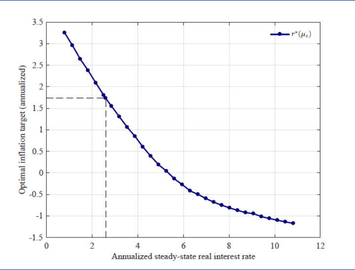
ECB Forum on Central Banking, November 2020
153
interestingly, the slope of the (r*, π*) locus around that value is quite steep (-0.9),
implying that a decline of r* of 1% relative to its baseline value is associated with an
increase in the optimal inflation target of 0.9%. Thus, we see that an inflation target
"below, but close to, 2%" is sub-optimally low for any value of r* below 2%. In
particular, the optimal inflation target corresponding to a value for r* of 1% (arguably,
at the higher end of current estimates of that variable) is close to 3%, well above the
ECB's current inflation target.
Chart 1
Optimal inflation target and real interest rate
Source: Andrade, Galí, Le Bihan and Matheron (2021). See text for description.
The findings summarized in Chart 1 are conditional on a policy rule that is meant to
capture the current state of affairs at the ECB, incorporating the effects of forward
guidance (i.e. "lower for longer" policies) consistent with a shadow rate rule with
historical estimates of the degree of inertia. So one may wonder if certain changes in
that rule would lead to an implied optimal inflation target closer to the ECB's current
inflation target given r* values of 1% (or lower). In Andrade et al. (2021) we analyze
several alternative rules with that purpose in mind. In particular, we consider an
interest rate rule identical to the estimated baseline rule except for the fact that the
ECB responds to average inflation over the past 4 or 8 years instead of inflation in
the current quarter. Once we condition on the previous average-inflation targeting
(AIT) rule our analysis of the optimal inflation target under r*=1% yields a value
slightly above 2% with 4-year averaging and slightly below 2% with 8-year
averaging. Thus, according to our estimated model, the adoption of AIT (with
sufficient memory) by the ECB would allow it to preserve the current inflation target,
if this was a priority. The same would be true, according to our analysis, if the ECB
rule were left unchanged, but a sizable emergency fiscal policy package was
ECB Forum on Central Banking, November 2020
154
implemented whenever the euro area experienced a large recession. In particular,
we show that if a fiscal rule was in place, whereby an increase in government
purchases corresponding to 4% of output is enacted when the cumulative output gap
reaches -6% and phased out through a 15% reduction per quarter, the optimal
inflation target under r*=1% would be about 2%. Of course, whether an aggressive
countercyclical fiscal policy rule of this sort is adopted lies beyond the decision scope
of the ECB.
While the previous examples illustrate the existence of alternatives to an increase in
the inflation target in the face of the decline in r* it is important to keep in mind some
of their limitations. In particular, in the case of AIT – a version of which has been
adopted by the Federal Reserve recently– most of its benefits hinge on the central
bank's credibility regarding its ability and willingness to keep inflation above target for
some time in order to make up for any eventual shortfall of inflation from target. And
only if such anticipation effects are at work in practice would an AIT rule display the
stabilizing gains (and hence the lower ELB incidence) that would allow it to maintain
the low current inflation target. That credibility may be questionable given that the
implementation of an AIT rule requires the central bank to be able to steer inflation
with precision towards a target that will be effectively moving over time.
Similar credibility issues may also loom over the adoption of a higher inflation target
by the ECB given the long period of inflation undershooting. However, in contrast
with AIT, the credibility problems in the case of a higher inflation target would be
restricted to the transition period, for once that target has been attained the ECB
could move on with a flexible inflation targeting rule that treats bygones-are-bygones
with no time inconsistent commitments needed. The potential transition problems
could be partly overcome through a gradual phase-in of the new regime. In
particular, the ECB could announce today that it may consider raising the inflation
target at some future time, but in no case before the current inflation target is
attained. Once the latter contingency materializes and, perhaps even better, once
inflation overshoots the current target (possibly as a result of some unexpected
supply shock), the ECB could announce its new (higher) target, and its intention to
attain it in the medium term. The fact that it would have pre-announced its intentions
to reconsider the target when inflation was much lower would neutralize any
criticisms of opportunism.
2 Concluding remarks
The decline in r* poses a major challenge to the ECB and other central banks. The
reason is simple: the value of r* is a key assumption in the design of a monetary
policy strategy. It was certainly an important assumption in the formulation of the
ECB strategy in 1998 and its review in 2003, respectively.
When a key assumption underlying a monetary policy framework is revised (as is the
case for the value of r*), the framework should be adjusted accordingly. Or else the
central bank should recognize the likely consequences of maintaining the current
framework, and explain the reasons for doing so in spite of those likely implications.
ECB Forum on Central Banking, November 2020
155
Making the current inflation target symmetric or adopting some sort of target range
may (or may not) be desirable moves by the ECB. But they represent a small tweak
of the current ECB framework and one that should not be viewed as a suitable
response to the decline in r*. The latter represents a major challenge that calls for a
significant adjustment that addresses that challenge effectively. A change in the
inflation target or in the rule followed to attain that target seems warranted.
References
Andrade, P., Galí, J., Le Bihan, H., and Matheron, J. (2021): "Should the ECB revise
its strategy in the face of a lower r*," CREI working paper 1767.
Brand, C. and Mazelis, F. (2019), "Taylor-rule consistent estimates of the natural rate
of interest", ECB Working Paper, No. 2057.
Eggertsson, G.B., Mehrotra, N.R. and Robbins, J.A. (2019), "A model of secular
stagnation: Theory and quantitative evaluation", American Economic Journal:
Macroeconomics, Vol. 11, No 1, pp. 1-48.
European Central Bank (2013), Background studies for the ECBs evaluation of its
monetary policy strategy, ECB, Frankfurt.
Holston K., Laubach, T., and J. Williams (2017): "Measuring the natural rate of
interest: International trends and determinants," Journal of International Economics
108, S59-S75.

ECB Forum on Central Banking, November 2020
156
Informal central bank communication
By Annette Vissing-Jorgensen
1
Abstract
Starting from a set of facts on the timing of stock returns relative to Federal Reserve
decision-making, I argue that informal communication – including unattributed
communication – plays a central role in monetary policy communication. This
contrasts with the standard communications framework in which communication
should be public and on-the-record because it serves to ensure accountability and
policy effectiveness. I lay out possible benefits of using unattributed communication
as an institution, but these should be weighed against substantial costs: it runs
counter to accountability to use unattributed communication, causes frustration
among those trying to understand central bank intensions, and enables use of such
communication by individual policymakers. Unattributed communication driven by
policymaker disagreements is unambiguously welfare reducing because it reduces
policy flexibility and harms the central bank’s credibility and decision-making
process. I suggest that central banks resist unattributed communication via
expensive newsletters and increase consensus-building efforts to reduce
disagreement-driven unattributed communication.
1 Facts: Information flows at unexpected times
I want to start with a set of facts to argue that central bank communication does not
always work the way you may think. The facts are about the Federal Reserve but, as
you will see, a lot of the underlying economics generalize to the ECB context.
Fact 1. Based on data from 1994 to 2011, Lucca and Moench (2015) document that
the average US stock return in the 24-hour period from 2 pm to 2 pm prior to
scheduled FOMC announcements was about 50 bps. They view this as a puzzle
since monetary policy news coming out would have to be systematically positive and
leaks are “unrealistic from an institutional viewpoint”.
Fact 2. Studying stock returns over the full cycle between scheduled FOMC
meetings, Cieslak, Morse and Vissing-Jorgensen (2019, CMVJ) document using
1994-2016 data that show stock returns (in excess of T-bill returns) on days that fall
in even weeks relative to the FOMC announcement day are on average 12 bps
higher than stock returns on days that fall in odd weeks. Chart 1 below illustrates
this, plotting 5-day average excess returns for days t to t+4 over the FOMC cycle.
CMVJ argue that this pattern is driven by monetary policy news, which over the post-
1
University of California Berkeley and NBER. I thank Adair Morse for many productive discussions.
ECB Forum on Central Banking, November 2020
157
1994 period has been unexpectedly accommodating (as opposed to generating a
risk premium). To link the stock return pattern to monetary policy, they document that
prior to 1994, when intermeeting target changes were common and thus reveal the
timing of Fed decision making/debate, these changes disproportionately took place
in even weeks in FOMC cycle time. This is shown in Chart 2 below.
2
CMVJ also
show that Fed funds futures yields on average fell in even weeks in FOMC cycle
time and that even-week stock returns were particularly high following low prior stock
returns, consistent with a surprisingly strong “Fed put”. They suggest that the even-
week timing of Fed news may arise from meetings/calls to discuss the discount rate
requests from the Federal Reserve Banks. These requests are themselves a
channel for influencing the target chosen at the next policy meeting. Each Reserve
Bank has to submit a request at least every two weeks, implying that a two-week
cycle for internal policy debate would be meaningful.
Chart 1
Stock returns over the FOMC cycle, 1994-2016
Source: Cieslak, Morse and Vissing-Jorgensen (2019).
2
The peaks in Chart 2 are delayed a couple of days relative to the peaks in Chart 1. Prior to 1994, the
FOMC did not make an announcement after the target was changed. The data source used in CMVJ
dates target changes based on when they were probably implemented in open market operations 1-2
days after the decision.
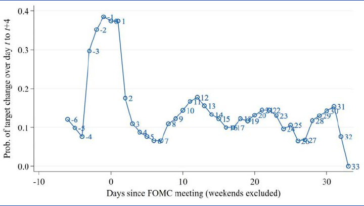
ECB Forum on Central Banking, November 2020
158
Chart 2
Target changes over the FOMC cycle 1982M9-1993M12
Source: Cieslak, Morse and Vissing-Jorgensen (2019).
Fact 3. Morse and Vissing-Jorgensen (2020, MVJ) studied the detailed calendars of
a set of Federal Reserve governors from 2007-2018. They document that even-week
returns are particularly high on days with interactions between governors and
Reserve Bank presidents, either at FOMC events or in phone calls or meetings.
Even-week days with governor-president calls/meetings see average stock returns
that are 15 bps higher than other even-week days. This implies that the pre-FOMC
period studied by Lucca and Moench (2015) is not special – even-week interactions
among top policymakers appear to more generally be associated with information
flow to markets. To document information flow via informal channels, MVJ document
that average stock returns on even-week days with governor-president interactions
are particularly high if there is informal communication via on-the-record public
commentary by the FOMC (using data from FOMC Speak) or governor calendars list
media interviews (of which almost none identifies the news outlet, suggesting they
are not on-the-record).
What is surprising about these stock return facts is that they are unaffected by
controlling for formal Fed communication: there are no formal communications
during the pre-FOMC period as it is part of the blackout period, and CMVJ and MVJ
find that controlling for speeches and formal information releases (e.g. Fed minutes)
does not materially affect the results. This suggests that monetary policy news
reaches markets via more informal channels.

ECB Forum on Central Banking, November 2020
159
Several pieces of evidence suggest a substantial role for unattributed
communication:
3
• CMVJ provide a series of examples of how confidential information from the
Fed has appeared in newspapers or market newsletters. They discuss how the
FOMC statement resulted from congressional pressure for transparency
following a series of newspaper stories revealing confidential Fed information.
• Former Governor Meyer’s 2004 book states: “The use of reporters as part of
the Fed’s signal corp is not official Board or FOMC doctrine. The public affairs
staff and the Chairman like to pretend it doesn’t happen.”
• Greg Ip, a top reporter covering the Fed for the Wall Street Journal and the
Economist, was asked in a 2012 interview whether he does a lot of “on-
background” interviews. He replied: “Yes, I do tons of them. With the Federal
Reserve, for example, it’s always been that way.”
4
• A comment by President Plosser at the January 2011 FOMC meeting is also
informative: “My impression is that the Board, for example, gives very few on-
the-record interviews, and, instead, the discussion is oftentimes on
background.”
This evidence begs the question of whether the transmission of monetary policy
news via unattributed communication is how monetary policy communication is
supposed to work.
2 The traditional view of monetary policy communication
Monetary policy is typically delegated to a central bank with some level of
independence from elected politicians. This is done to ensure that the central bank is
able to implement policy that may be unpopular but necessary, like raising rates or
imposing macro-prudential rules.
5
Furthermore, the complexity of central banking
makes it a governmental function best delegated to an agency of experts. The role of
communication in this setting is twofold.
3
A multitude of terms are used in journalism to describe how information can be used by the reporter.
“On-the-record” means that everything is usable and the source can be quoted by name. “Off-the-
record” means the information obtained cannot be used for publication. In between there is a range of
categories for which definitions vary. Using the Fed’s interpretation, based on Meyer (2004), “not for
attribution” means everything is usable, the source should not be directly identified, but the information
can be attributed to “senior Fed officials” or the like. “On background” means information gathered can
be used but not attributed to the official directly or the Federal Reserve but to “government officials” or
similar. “On deep background” implies that information is usable but no source information should be
given. I will use “unattributed” to refer to “not for attribution”, “on background” and “on deep
background”.
4
https://journalistsresource.org/tip-sheets/research/chat-the-economists-greg-ip-key-tips-business-
reporting-analysis/
5
Bernanke (2015) describes the unpopularity of the AIG bailout and states: “If we acted, nobody would
thank us. But if we did not act, who would? Making politically unpopular decisions for the long-run
benefit of the country is the reason the Fed exists as a politically independent central bank. It was
created for precisely this purpose: to do what must be done – what others cannot or will not do.” The
AIG example documents that even expansionary policies can be widely unpopular.

ECB Forum on Central Banking, November 2020
160
Accountability, to sustain independence. A central bank needs to convey the gist
of its deliberations to elected parliamentarians and the public so they can ensure that
decisions are made competently in accordance with the central bank’s mandate.
Some of this communication is invariably technical in nature. However, the central
bank’s independence from political pressure is more likely to endure if the broad
public understands decisions and views the central bank as competent.
Policy effectiveness. The impact of forward guidance and asset purchases on
medium and long interest rates depends crucially on the public understanding the
likely duration of low rates/monthly purchases. Furthermore, effective monetary
policy requires economic agents (households, firms, governments) to understand the
central bank reaction function. For example, agents will behave less conservatively
in their spending decisions (C, I, or G) if they understand that the central bank will
accommodate aggressively if needed.
3 On-the-record versus unattributed communication
The traditional roles for communication suggest that communication should be public
and on-the-record, conveying the central bank’s chosen policy and policy framework,
and allowing oversight by all who want to hold the central bank accountable.
Possible explanations for why unattributed communication plays a role can be
grouped into two categories.
6
1. The Federal Reserve as an institution may prefer unattributed to on-the-record
communication in some situations.
2. Unattributed communication could be driven by disagreeing policymakers who
each try to influence the expectations of the public or financial markets in order
to strengthen their bargaining position at the Fed.
Let me consider each possibility in turn.
4 Institutional use of unattributed communication
4.1 Benefits of unattributed institutional communication
The political science literature is at the forefront of knowledge about unattributed
communication since such practices are standard in politics. Pozen (2013) focuses
on leaks from the White House and argues that many of these are not leaks in the
sense of unauthorized disclosure but are instead authorized “plants” of information in
6
I am disregarding the possibility that the documented return patterns are due to policymakers
inadvertently disclosing large amounts of information, given the pervasive nature of information flow
implied by the asset pricing evidence reviewed. I am also not going to discuss the very unlikely
possibility that someone inside the Fed with access to the information is systematically trading on it.

ECB Forum on Central Banking, November 2020
161
media outlets. The use of plants rather than for-attribution disclosure allows the
sender to “impart information about executive branch policies without officially
acknowledging those policies and thereby inviting unwanted forms of accountability
or constraints”. Mapping this to the central banking context, the benefits of
unattributed communication include the following.
Flexibility: In the Fed context, it is beneficial to provide frequent policy guidance in
order to facilitate more accurate decision-making by the private sector. However,
communication ties policymakers’ hands if the public does not fully understand the
state-contingent nature of policy. In that case, the Fed will be viewed as flip-flopping
if policy differs from prior statements of likely outcomes. Unattributed comments may
impose less of a constraint on subsequent policy decisions than on-the-record
communication (since less of a promise has been made), though of course more
than no communication at all.
Consistent with the idea that the Fed is very concerned about policy flexibility and
views formal disclosure as especially flexibility-reducing, the Fed used to delay the
release of minutes until after the subsequent FOMC meeting in order to “safeguard
the Committee’s flexibility to make needed adjustments to policy” (Vice Chairman
Kohn, July 1993 FOMC meeting). Furthermore, in 1994 the Fed agreed to make
public statements if policy is changed. This action coincided with an abrupt reduction
in the frequency of intermeeting rate changes, from about 2/3 to around 10% of all
changes (see CMVJ). This has to my knowledge never been explained but is likely to
be due to an aversion to make formal public statements for fear that they will tie the
committee’s hands going forward (in particular, by making it hard to reverse an
intermeeting change for fear of looking less competent). Vissing-Jorgensen (2019)
provides quotes from the FOMC transcripts to further document the importance of
policy flexibility and how it is reduced by Fed disclosure.
Explaining: Use of unattributed communication could also be motivated by a Fed
desire to explain its assessment of the economy and its policy or policy framework.
Using background conversations with reporters is less time-consuming than on-the-
record communication since it does not require the Fed to engage in a subsequent
public debate about the information disclosed.
Learning: Another possibility is that unattributed communication via “plants” is used
for learning purposes: to gauge support outside the Fed for a particular policy
change (or economic assessment). This is what the political scientists refer to as a
“trial balloon leak”. By floating an idea not-for-attribution, the Fed avoids looking bad
if the idea is unpopular and not implemented. A Wall Street Journal article discusses
how Bernanke appears to have floated the idea of doing Operation Twist with a
market newsletter in August 2011 to test the waters.
7
These are all meaningful benefits, but unattributed communication has costs.
7
https://www.wsj.com/articles/SB10001424052970204554204577025922155198762

ECB Forum on Central Banking, November 2020
162
4.2 Costs of unattributed institutional communication
Unattributed communication is the opposite of transparency and
accountability: In a time of populism, public appreciation of the role and tools of
central banks is crucial for these to retain their legitimacy and independence. The
Bank of England’s Citizens’ Panels, the “Fed Listens” events, and the “ECB Listens”
events that are part of the ECB’s review exemplify recent initiatives to increase
transparency and accountability by engaging in direct communication with the public
at large. Yet, the lack of public understanding of Federal Reserve informal
communication stands in stark contrast to such efforts. I wonder what the newly-
engaged citizens would think if we told them that the Federal Reserve, and perhaps
other central banks, does a lot of its communication in ways that are not well
understood but appear to have enormous impact on asset prices. I suspect they
would worry about who gets access to all that information first and how their pension
fund managers are doing in that race. Certainly, their trust in central banks as
institutions would not increase.
8
Frustration: It is likely that the level of frustration with Fed communication is higher
if market participants are in a constant struggle to understand which newsletters and
newspapers have obtained new information from the Fed. Is the Fed putting itself in
a situation in which thousands of frustrated market participants and reporters are
ready to criticize the Fed following any decision or announcement that appears
inconsistent with prior perceptions?
9
In this sense, using unattributed communication
may actually reduce policy flexibility, relative to on-the-record communication. Use it
sparingly! It may come back to haunt you.
One could formalize this possibility as follows. Think of a setting in which today is
date 0 (say half way through the policy cycle) and the central bank’s next policy
meeting is at date 1. Express the credibility cost to the Fed of setting a policy rate
at date 1 that differs from what the market expects after any date 0 disclosure as:
×
[
(
)
]
where
=
[Formality of date 0 disclosure] + [Frustration with Fed communication]
Understanding of reaction function
If the public has a complete (infinite) understanding of the Fed’s reaction function,
market expectations do not constrain policy – is zero since the public will
8
A quote by Mr Fisher, Manager of the Fed’s System Open Market Account, summarizes his frustration
with the Fed’s communication giving unfair information access to some. Referring to market
movements in the intermeeting period leading up to the June 1999 FOMC meeting, he states: “In my
judgment, if you had tried to trade in the bond market during this period and had followed only the
FOMC’s announcement on May 18, the data releases as they came out, and the Chairman’s Joint
Economic Committee testimony, you would have lost a lot of money. On the other hand, if you had
subscribed to all the high-priced insider rags and carefully tracked the utterances, attributed and
unattributed, of FOMC members, you would have fared a good bit better.”
9
We can argue about whether off-the-record communication enhances the understanding of the reaction
function relative to on-the-record communication. Perhaps policymakers are willing to say more about
the reaction function when they can use informal communication, though a confident central banker
should be happy to speak on-the-record.
ECB Forum on Central Banking, November 2020
163
understand that news arrived between date 0 and 1 that necessitates a different
policy rate. If not, communication matters. The flexibility argument is that less formal
announcements retain more flexibility, here captured by [Formality of date 0
disclosure] and thus being lower. However, this ignores any indirect effects of
disclosure choice on the frustration term. Accounting for that, unattributed
communication may retain less flexibility than on-the-record communication.
Facilitates use by individual policymakers: By using unattributed communication
as an institution, the Fed opens itself up more to the tug-of-war over market
expectations by disagreeing policymakers. With less clear institutional guidance on
how the consensus is evolving, individual policymakers have more room to try to
drive market expectations.
5 Individual policymaker use of unattributed communication
Rather than being used for institutional communication, the second possible driver of
unattributed communication is that individual policymakers seek to gain influence
from using it. Disagreement about appropriate policy is a central feature of group
decision-making and it places monetary policymaking in a more standard political
setting. Central bank communication in a setting with disagreement is not only
institutional but also individual. It becomes about affecting markets and public
opinion to improve your bargaining position in policy negotiations.
5.1 Individual communication
An individual policymaker may seek to gain from changing public views in several
ways.
Posturing: Making firm statements of what policy the policymaker prefers. This
imposes a greater loss from compromise on the policymaker him/herself, thus
improving his/her bargaining position. Posturing is clearly best done via public on-
the-record communication in speeches or interviews.
Influencing: Changing the public’s view of appropriate policy by putting forward
arguments supporting the policymaker’s view. This makes it costlier for other
policymakers to deviate from the policymaker’s preferred policy.
Spin: Distorting the public’s assessment of what the likely policy decision is. Those
succeeding in moving the public’s expectations in their preferred direction gain
bargaining position because the central bank as an institution (and thus all central
bank policymakers) suffer if the central bank is perceived as flip-flopping. Any
perceived lack of competence plays into the hands of politicians seeking to reduce
central bank independence.
The line between influencing and spin is thin. Both are intended to affect beliefs, but
spin implies the use of more manipulative tactics to control the message. Crucially, if
influencing or spin is based on confidential information, it has to be done using

ECB Forum on Central Banking, November 2020
164
unattributed communication. In central banking, staff economic projections, internal
deliberations, and views of colleagues are often confidential until a decision has
been made (or in some cases much longer).
10
11
5.2 The game theory of unattributed individual communication
In Vissing-Jorgensen (2019) I model the unattributed tug-of-war over market
expectations between disagreeing policymakers, what one could call the “quiet
cacophony”. In the model, two policymakers set policy.
• Each policymaker’s preferred policy rate evolves over time. Policymakers know
each other’s preferred rate at each point in time. They choose what to reveal to
the public about policy preferences at an intermediate date between policy
meetings. Policymakers care about how close the chosen policy rate is to their
preferred rate but also about the central bank not being viewed as “flip-
flopping”. If either policymaker communicates with the public, both incur a loss if
the chosen policy rate deviates from the average preferred policy rate
communicated at the intermediate date. Providing information at the
intermediate date about policymaker preferences thus reduces policy flexibility.
• If no information is provided to the public, the chosen policy rate at the next
meeting is the average of policymakers’ preferred rates at that time.
• With communication, the chosen policy rate is a weighted average of the
average preferred policy rate at the time of the meeting and the market’s
expectation of the average preferred policy rate based on information
communicated at the intermediate date.
Given all this, will policymakers decide to disclose information about policy
preferences at the intermediate date and what will they disclose?
• Assume that policymakers are to some extent able to spin market perceptions
of policy preferences by selectively revealing internal information that supports
a claim that policymakers’ average preferred policy rate is higher (or lower) than
is in fact the case.
The outcome of the game is that if disagreement is sufficiently strong (judged
relative to the amount of news that may arrive before the next policy meeting)
and sufficient spin is possible, the unique Nash equilibrium is that each
policymaker communicates with his/her preferred spin in order to move the
policy rate chosen in his/her preferred direction.
10
The FOMC Policy on External Communications of Committee Participants lays out what is confidential,
see https://www.federalreserve.gov/monetarypolicy/files/FOMC_ExtCommunicationParticipants.pdf
11
There are also instances where the identity of the messenger affects the impact of the message. For
example, hearing that a known policy hawk thinks inflation is just around the corner may affect public
opinion less than a press article stating that some central bank officials privately worry about the risk of
inflation.

ECB Forum on Central Banking, November 2020
165
Chart 3 below illustrates how each policymaker’s spin reacts to that of the opponent.
In the example graphed, person D’s preferred policy rate is lower than that of person
H. If H does not spin, D therefore spins the market’s expectation of the average
preferred policy rate negatively (point A in the chart). If H does spin, he will spin
positively given his policy preference. The more positively H spins, the more
negatively D spins to counter. In equilibrium, we thus end up at point B where both
spin to the fullest extent possible (S* and –S*) but the spin cancels out.
Since the spin cancels out, neither policymaker gains from their communication.
However, the disclosure reduces (compared to no disclosure) the flexibility of the
central bank to react to information arriving between the intermediate date and the
next policy meeting. As a result, both policymakers are worse off than if they could
each commit to not using informal communication. This provides an illustration of
welfare-reducing use of unattributed communication. It is an analogue to the
prisoners’ dilemma, in which both prisoners would be better off if neither confessed
(to get a reduced sentence) but both confess in equilibrium.
Chart 3
The tug of war over market expectations: Spin reaction functions
Source: Vissing-Jorgensen (2019).
In the model described, both parties are equally able to spin, implying that spin
cancels in equilibrium. One could think of cases in which the internally known
information all (or mainly) favours one side, with the other side unable to counter.
Two recent disclosures of ECB staff projections the day before scheduled policy
announcements exemplify this.

ECB Forum on Central Banking, November 2020
166
• A September 11, 2019, a Reuters article titled “ECB projections to show future
growth barely above 1%: sources” illustrates a dovish leak, motivated by a
desire for additional policy accommodation. It states: “Growth will be not far
above 1 percent both this year and next, the charts are expected to show,
underpinning the ECB’s plans to approve more stimulus, the sources, who
asked not to be named, told Reuters.”
12
• A September 9, 2020 Bloomberg article titled “ECB Forecasts Said to Show
More Confidence in Economic Outlook” illustrates a hawkish leak. It attributes
information about the forecast to “euro-area officials” who “also said that in their
view additional monetary support beyond the current 1.35 trillion-euro ($1.6
trillion) emergency bond-buying program doesn’t appear warranted from the
current perspective”.
13
In these examples, those communicating may benefit in the short run by an
improved bargaining position at the policy meeting, but on average over time each
side gains as often as they lose.
14
Harm to credibility and the decision-making process: In Vissing-Jorgensen
(2019), I study FOMC transcripts back to 1948 to gain insight into whether
unattributed communication has other costs than lost policy-flexibility relative to non-
disclosure. The Fed uses the word “leak” for non-institutionally sanctioned
communication of confidential information. I document 114 FOMC documents with
discussions of leaks (generally one document corresponds to one FOMC meeting or
conference call). The documents reveal that such communication is viewed as a
threat to Fed credibility and harms the Fed’s decision-making process. For example,
a 2010 memo from Chairman Bernanke to the FOMC states: “[...] it damages the
reputation and credibility of the institution if the outside world perceives us as using
leaks and other back channels to signal to markets, to disseminate points of view, or
to advance particular agendas” and “such leaks threaten the free give and take of
ideas and collegiality of the FOMC as we grapple with the difficult issues we face”.
In addition to leaks harming the free give and take of ideas, the withholding of
information to prevent leaks further damages decision quality. Meyer (2004)
describes how staff used to omit information from the Greenbook for fear of leaks by
policymakers. A 2014 Reuters article gives an example of information withholding at
the ECB, stating that “Several ECB sources said Draghi had cut back on circulating
policy papers in advance of council meetings, apparently out of concern that
12
https://www.reuters.com/article/us-ecb-policy-forecasts/ecb-projections-to-show-future-growth-barely-
above-1-sources-idUSKCN1VW259
13
https://www.bloomberg.com/news/articles/2020-09-09/ecb-forecasts-said-to-show-more-confidence-in-
economic-outlook
14
An interesting aspect of the game-theoretic framework is that as the policy decision nears, the
temptation to disclose internal information (via unattributed communication) increases since the benefit
of retaining flexibility to better react to any new information that may arrive before the decision
diminishes.

ECB Forum on Central Banking, November 2020
167
opponents, notably in the German Bundesbank, were leaking them to try to block or
discredit decisions.”
15
This could materially harm the quality of decisions made.
6 Suggestions
6.1 Resist communicating via expensive Fed-watcher or ECB-watcher
newsletters whether for individual or institutional reasons
The Medley Global Advisors scandal in 2012 that led to the resignation of President
Lacker from the Richmond Fed was very harmful to the Fed’s reputation. It
reinforced concerns about unequal access to information. When I tried to buy the
Medley newsletter a few years ago, it cost $120,000/year. Yes, it is easier for central
bankers to convey what they want to experts via newsletters, and the newsletter can
drive market expectations quickly, but so can financial newspapers.
In a time when trust in formal institutions is low, populism is prevalent, and
governments are under pressure to finance huge deficits, central bank independence
cannot be taken for granted. A new paper by Bianchi, Kind and Kung (2020)
documents significant drops in Fed funds futures rates around Trump tweets about
the Fed. How many more Medley scandals can Fed independence take?
6.2 Seek consensus to avoid the prisoners’ dilemma of disagreement-
driven unattributed communication
At the ECB, President Lagarde has introduced a series of changes to limit
unattributed communication driven by disagreements. A February 2020 Reuters
article titled “No phones, no leaks: How Lagarde is making her mark on ECB”
describes the changes.
16
The changes in phone use are useful and make for a good
headline, but other changes are likely more important. They include the president
spending more time listening to colleagues, building consensus, not front-running
decisions before meetings, and showing more trust in colleagues by distributing
meeting proposals up to a week in advance, not just hours before for fear of leaks.
How do these changes relate to the prisoners dilemma? Standard solutions include
enforcement (in a military context, think of arms treaties with inspectors) or
punishment in a repeated version of the game. The new no phones policy fits in the
enforcement category but only helps for information obtained during the meetings.
The consensus-building approach maps directly to the repeated game solution, since
the President now has the choice to take away influence if someone leaks. This
cannot work perfectly, since leakers are hard to identify. However, an improved
15
https://www.reuters.com/article/us-ecb-governors-exclusive/exclusive-central-bankers-to-challenge-
draghi-on-ecb-leadership-style-idUSKBN0IO1GY20141104
16
https://www.reuters.com/article/us-ecb-policy-lagarde-inisght/no-phones-no-leaks-how-lagarde-is-
making-her-mark-on-ecb-idUSKBN2040NO
ECB Forum on Central Banking, November 2020
168
consensus-focused culture is likely to make leaking less acceptable among
colleagues who may know the identity of a leaker. While they may not formally want
to reveal this, they can help impose informal sanctions. After all, many policymakers
will see their influence reduced if the President goes back to a less consensus-
building approach. Pozen (2013) describes in the US political context how leakers
are disciplined informally via “shaming, shunning and exiling”.
References
Bianchi, F., Kind, T., and Kung, H. (2020), “Threats to Central Bank Independence:
High-Frequency Identification with Twitter”, working paper.
Cieslak, A., Morse, A., and Vissing-Jorgensen, A. (2019), “Stock Returns over the
FOMC Cycle”, Journal of Finance, 74, 7, 2201-2248.
Lucca, D. O. and Moench, E. (2015), “The Pre-FOMC Announcement Drift”, Journal
of Finance, 72, 1, 329-371.
Morse, A. and Vissing-Jorgensen, A. (2020), “Information Transmission from the
Federal Reserve to the Stock Market: Evidence from Governors’ Calendars”, working
paper.
Pozen, D. E. (2013), “The Leaky Leviathan: Why the Government Condemns and
Condones Unlawful Disclosures of Information”, Harvard Law Review, 127, 512-635.
Vissing-Jorgensen, A. (2019), “Central Banking with Many Voices: The
Communications Arms Race”, Conference Proceedings, 23rd Annual Conference of
the Central Bank of Chile.

ECB Forum on Central Banking, November 2020
169
The decline in euro area inflation and
the choice of policy strategy
By Volker Wieland
1
Abstract
This note argues that the European Central Bank should adjust its strategy in order
to consider broader measures of inflation in its policy deliberations and
communications. In particular, it points out that a broad measure of domestic goods
and services price inflation such as the GDP deflator has increased along with the
euro area recovery and the expansion of monetary policy since 2013, while HICP
inflation has become more variable and, on average, has declined. Similarly, the cost
of owner-occupied housing, which is excluded from the HICP, has risen during this
period. Furthermore, it shows that optimal monetary policy at the effective lower
bound on nominal interest rates aims to return inflation more slowly to the inflation
target from below than in normal times because of uncertainty about the effects and
potential side effects of quantitative easing.
1 The challenge
In her recent speech at the conference “The ECB and its Watchers XXI”
2
the
President of the European Central Bank, Christine Lagarde, pointed out the following
major challenge that would need to be addressed by the ECB strategy review:
“Most importantly, the last decade has been defined by a persistent decline in
inflation among advanced economies. In the euro area, annual inflation averaged
2.3% from 1999 to the eve of the great financial crisis in August 2008, but only 1.2%
from then until the end of 2019. … We need to thoroughly analyse the forces that are
driving inflation dynamics today, and consider whether and how we should adjust our
policy strategy in response.”
3
This note aims to contribute some suggestive findings concerning possible driving
forces for inflation dynamics in the past and in the future and to discuss aspects of
an appropriate policy strategy.
1
Institute of Monetary and Financial Stability at Goethe University of Frankfurt and German Council of
Economic Experts (GCEE). Helpful comments and analysis by Jens Herold, Lars Other, Milena
Schwarz, Chih-Chun Huang and Sebastian Weiske are gratefully acknowledged. Remaining errors are
the author’s responsibility.
2
The conference that was held in Frankfurt on September 30, 2020 also formed part of the ECB Listens
events in the context of the ECB Strategy Review. It is part of a conference series organised by the
Institute for Monetary and Financial Stability. See www.imfs-frankfurt.de.
3
See Lagarde (2020).

ECB Forum on Central Banking, November 2020
170
2 Inflation measures indicate important role of import prices
in the decline of consumer price inflation
As a first step, this note looks into four measures of inflation averages in the euro
area between 1999:Q1 and 2020:Q1 (See Table 1). Somewhat differently from the
reference provided in President Lagarde’s speech the timeline is divided into three
periods to better distinguish inflation dynamics during economic recession and
recovery. The first period runs from 1999:Q1, when the monetary union was
launched, up to 2009:Q1, when the union recorded a sharp decline of GDP. The
second period is set between 2009:Q2 and 2013:Q1, that is, from the business cycle
trough during the financial crisis to the trough of the euro area debt crisis. The third
period, between 2013:Q2 and 2020:Q1, marks the subsequent economic recovery.
The four inflation measures are 1) the Harmonized Consumer Price Index (HICP),
which was referred to by President Lagarde, 2) the HICP excluding energy prices, 3)
the GDP deflator, which covers prices of all goods and services produced in the euro
area and 4) the import price deflator, which accounts for the inflation in imported
goods and services prices.
Table 1
Inflation averages
(% growth rates)
Inflation measures
Q1 1999 – Q1 2009
Up to financial crisis
recession
Q2 2009 Q2 – Q1 2013
Financial crisis and euro
debt crisis recessions
Q2 2013 – Q1 2020
Economic recovery up to
coronavirus recession
HICP: Harmonized index of
consumer prices
2.2 1.8 0.9
HICP excluding energy
prices
2.0 1.4 1.1
GDP Deflator: Domestic
goods price inflation
2.0 1.0 1.3
Import price deflator: Import
price inflation
1.6 2.1 -0.3
Sources: Eurostat, ECB.
In the first period, the results for the HICP and the GDP deflator are very similar. The
HICP averaged 2.2 %, while excluding energy prices results in an average of 2.0%.
Domestic goods price inflation measured by the GDP deflator was also on average
2.0%. Yet, the GDP deflator is quite a different measure of inflation compared with
the HICP. First of all, it is not based on a particular goods and services basket but on
actual expenditures. Furthermore, it is quite a bit broader in coverage because it also
includes prices of investment goods produced in the euro area, prices of construction
investment, prices of exported goods and services, as well as prices of public goods
and services. It excludes prices of imported goods and services. Thus, it is the
broadest possible measure of domestic goods price inflation. Imported goods price
inflation averaged only slightly lower at 1.6% throughout this period. This includes
imports for consumption and investment purposes by households, firms and public
sector entities, as well as imports of intermediate goods used in the production of
exports.
ECB Forum on Central Banking, November 2020
171
Splitting the post-2009 period of the monetary union into two makes quite a
difference relative to the observations made by President Lagarde in her speech.
First, the HICP stays high on average at 1.8% between 2009:Q2 and 2013:Q1 while
fluctuating much more strongly than in the preceding period. From 2013:Q2 to
2020:Q1, average HICP inflation is quite a bit lower at 0.9%. This is puzzling,
because macroeconomic theory as well as past empirical observation would suggest
that inflation is low in periods of recession while increasing along with economic
recovery. The recent experience in the euro area is the opposite, at least as far as
the HICP measure of inflation is concerned. Much of the volatility in HICP is due to
energy prices. In fact, the standard deviation of HICP inflation excluding energy
prices is largely unchanged at about 0.4% before and after the financial crisis.
Nevertheless, the HICP excluding energy prices also exhibits a somewhat
counterintuitive pattern of averages, with 1.4% during the double-recession period
and 1.1% during the subsequent recovery period.
Domestic goods price inflation measured by the GDP deflator, however, is quite
different on average. It came in substantially lower during the double-recession
period at 1.0% and then averaged 1.3%. While this is not a large increase on
average, it goes at least in the right direction as inflation increases in the economic
recovery. Import prices help explain the difference between the HICP and the GDP
deflator. As measured by the import deflator, import price inflation averaged 2.1%
during the double recession, but fell to an average of -0.3% during the recovery.
Note that the difference between the HICP and GDP deflator cannot be explained by
the prices for oil and natural gas imports alone, as the HICP excluding energy prices
also showed the opposite pattern with higher inflation during recession than during
economic recovery. It would be of interest to estimate the import components of
consumption expenditure in order to gain a deeper understanding of consumer price
inflation excluding import prices. Unfortunately, national income accounts do not
provide a decomposition of imports according to consumption, investment or other
purposes.
Chart 1 shows the timeline for inflation measured with the HICP and the GDP
deflator. Up to about 2007 the two measures provide a very similar picture of inflation
dynamics. Afterwards, the HICP becomes much more volatile. The average is still
high during the double-recession period because it increases towards 3% between
2011 and 2012. From 2014 onwards it fluctuates between a marginal dip into the
negative territory and 2%. By contrast, the GDP deflator stays near 1% in the
double-recession period and rises during the recovery period, eventually reaching
1.7% in 2019. This would roughly correspond to the ECB’s numerical target of “close
to but below” 2%. Bletzinger and Wieland (2017) estimate a symmetric numerical
target at 1.74% based on an interest rate reaction function that fits ECB interest rate
decisions from 1999 to 2013 quite well. Yet, of course, the ECB’s target is formulated
with respect to the HICP and not to the GDP deflator.
From 2013 onwards the ECB lowered the main refinancing rate towards zero and
engaged in substantial further policy easing by means of targeted longer-term
refinancing operations, as well as massive quantitative easing (QE) by the means of
direct asset purchases. It is not easy to estimate the effect these measures have had
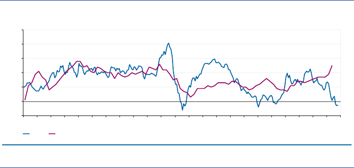
ECB Forum on Central Banking, November 2020
172
on HICP inflation due to its volatile nature. By contrast, the sustained increase in the
GDP deflator matches up better with the economic recovery from 2013 onwards and
the substantial policy easing conducted till 2018. Thus, taking a broader look at
domestic price inflation in terms of the GDP deflator also helps in pointing out the
effects of the ECB’s policy.
Chart 1
Growth rates of HICP and GDP deflator in the euro area
(percentage)
Sources: ECB, Eurostat
In 2020, domestic price inflation increased further, reaching 1.9% in Q1 and 2.5% in
Q2. In the meantime, HICP inflation collapsed and slid into negative territory in the
fall. This decline is associated with a sharp drop of import prices, that are partially
included in the HICP but excluded from the GDP deflator. Unfortunately, the GDP
deflator only becomes available with a delay. The increase to 2.5% in the second
quarter of 2020 is partly due to increased public sector inflation, mostly in France.
This is driven by the accounting for the large-scale shutdown in response to the
coronavirus pandemic. Country-level data that has so far become available for
2020:Q3 indicates lower readings of about 1.1% for Germany and France in that
quarter.
Currently, ECB strategy and communication is focused almost exclusively on the
HICP and core HICP measures. Yet, in order to better understand and explain the
forces driving inflation since the global financial crisis it would appear helpful to take
a broader look at inflation measures. This includes, in particular, domestic goods
price inflation as captured by the GDP deflator. In recent years its dynamics have
been somewhat more closely aligned with the business cycle and with monetary
policy expansion than HICP inflation.
-1
0
1
2
3
4
5
1998 99 00 01 02 03 04 05 06 07 08 09 10 11 12 13 14 15 16 17 18 19 2020
Year-on-year change in %
HICP GDP deflator
2
1 – Working day and seasonally adjusted. 2
– Quarterly data.
ECB Forum on Central Banking, November 2020
173
3 Effects of housing cost and climate policy on consumer
price inflation
3.1 Rental cost and owner-occupied housing
A key element of the cost of living is housing cost which, however, is understated in
the HICP, as the index includes only rental housing cost and ignores owner-occupied
housing cost. This is a serious omission since the latter accounts for a large share of
dwellings in the euro area: 50% in Germany and 70% or even higher in most of the
member states in the currency union (Brunßen and Diehl-Wolf, 2018). Contrary to
the HICP, the Consumer Price Index (CPI) for Germany includes owner-occupied
housing cost and uses the rental-equivalency approach to estimate it. Rents for
comparable rental housing are used to account for the costs of owner-occupied
housing. As a result, a change in rental cost, including owners’ equivalent rent, in the
German CPI, is similar to a change in the actual rents considered in the German
HICP. But rental cost receives essentially double weight in the CPI due to the
inclusion of owner-occupied housing. The annual increase in rental costs in the CPI
and in the HICP has averaged at 1.36% and 1.42% respectively since 2013. By
comparison, the CPI increased by 1.16% per year and the HICP by about 1.21%.
While rents increased more than the overall measures of inflation, the CPI
nevertheless rose a little more slowly than the HICP for Germany. This is due to
other differences. Yet there can be stronger effects on the HICP at particular points in
time due to the smaller weight on rental costs. For example, in October 2020 the
year-on-year rate for the CPI stood at -0.2% while that of the HICP came in at -0.5%
and the early release for November indicates -0.3% and -0.7% respectively.
The rental-equivalency approach is also used in the Netherlands but not in most
other euro area member states. It is argued that the share of rental housing is too
small to provide sufficiently good grounds for comparison. Yet the consumer price
index for the United States, which has a home ownership rate of about 65%, also
includes owners’ equivalent rent of primary residence (OER) (Bureau of Labor
Statistics 2020). An estimate is obtained by means of a survey, in which
homeowners are asked how much they would charge monthly if leasing their home
unfurnished and without utilities. Since 2014, rent and owners’ equivalent rent in the
U.S. have grown at rates above 3% and have contributed to the rise in U.S. inflation.
By 2018 underlying inflation as measured by the CPI excluding food and energy was
stable at 2% in the United States compared to, in the euro area, 1% in HICP
excluding energy, food, alcohol and tobacco and 1.2% in HICP excluding energy and
unprocessed food. Part of the reason was the greater increase in rents and the
additional weight given to owners’ equivalent rent in the U.S. CPI (see also
Grossmann-Wirth and Monette 2017 and Gros 2018).
Turning to the euro area, Chart 2 shows that actual rent inflation included in the
HICP is much more stable than inflation measured by the HICP excluding energy.
Inflation in the latter swings up and down from actual rent inflation. If a rental-
equivalency approach were to be used for owner-occupied housing, then at least the
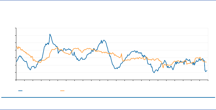
ECB Forum on Central Banking, November 2020
174
weight on rent inflation in the HICP would increase substantially, presumably to more
than double the current weight. As a result, variation in the HICP excluding energy
would be reduced and, presumably, show less of a decline at the current juncture.
Furthermore, since 2013 the rent inflation component included in the HICP has
averaged at 1.25% annually compared to 1.10% in the HICP excluding energy. Thus,
if owners’ equivalent rent has increased at a similar rate to the actual rents, the
inclusion of owners’ equivalent rent is expected to raise HICP inflation throughout
this period somewhat, but probably only a few basis points annually.
Chart 2
Growth rates of rents included HICP and HICP excluding energy
Actual rentals for housing and HICP excluding energy: Euro area
(percentage)
Sources: ECB, Eurostat, own calculations:
For a number of years, Eurostat has been developing new indices for owner-
occupied housing (OOH price index) in partnership with national statistical offices.
These indices are based on a net acquisition approach (European Commission,
2018) which focuses on actual monetary transactions and consumption
expenditures. Thus, it is closer to the method used for the HICP in general. This
method records the change over time of all expenditure incurred in the acquisition of
housing, as well as purchase of goods and services related to housing.
Owner-occupied Housing Price Index (OOHPI) data are being prepared for most of
the member states in the euro area but the statistics for the currency union as a
whole are not available. Chart 3 shows OOHPI inflation for Germany, France, Italy
and Spain. In contrast to rents, the net acquisitions cost of owner-occupied housing
varies considerably across the four countries. In Germany, growth rates rose steadily
from 2% in 2014 to about 5% by the end of 2018. In France, the growth rate of the
OOHPI fell from 5% in 2011 to about -2% in 2013 and then moved between 0% and
3% in the following years. In Italy, OOHPI inflation declined from about 3% in 2011 to
below -1% in 2014 and then stayed between 0% and 1% in recent years. The
decline, in the aftermath of the financial crisis, has been most dramatic in Spain,
where OOHPI inflation fell to -10% in 2012, then returned to positive territory in 2014
and rose to 6% by 2019.
0
0.5
1.0
1.5
2.0
2.5
3.0
3.5
1998 00 02 04 06 08 10 12
14
16 18 2020
Year-on-year change in %
HICP excluding energy
1
Actual rentals for housing in HICP
2
1 – Working day and seasonally adjusted. 2 – Not seasonally adjusted.
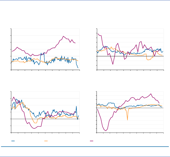
ECB Forum on Central Banking, November 2020
175
The development of OOHPI inflation after the financial crisis and its great variability
across the four countries suggests that the index exhibits some properties of an
asset price. Of course, it could be argued that the oil price, which plays a significant
role in the HICP, is also highly variable and exhibits asset price characteristics as it
depends on the relationship between oil demand and the available stock of oil in the
ground. However, to the extent that the net acquisitions approach includes the
purchase of land, it includes an asset that is not exhausted in the production of
housing services. Rather it remains available to the same extent for future housing.
The price of this asset needs to be excluded if one wants to include the cost of
owner-occupied housing in the consumer price index. The national accounts also
treat the structure of housing as investment rather than consumption. Yet, it certainly
has the aspects of a durable consumption good.
Chart 3
Owner-occupied housing indices and the HICP excluding energy
Cost of owner-occupied housing and HICP
(percentage)
Sources: Eurostat, own calculations.
Some practical concerns have been raised regarding the proposal to include the
OOH price index in the HICP (European Commission, 2018). In particular, the
OOHPI is published 100 days after the end of each quarter and has been subject to
major revisions. Thus, it has been suggested that this practice is not compatible with
the HICP, which is required to be published 15 days after the end of each month.
0
1
2
3
4
5
6
2011 12 13 14 15 16 17 18 19 2020
Germany
Year-on-year change in %
-3
-2
-1
0
1
2
3
4
5
6
2011 12 13 14 15 16 17 18 19 2020
France
Year-on-
year change in %
-2
-1
0
1
2
3
4
2011 12 13 14 15 16 17 18 19 2020
Italy
Year-on-year change in %
-12
-10
-8
-6
-4
-2
0
2
4
6
8
2011 12 13 14 15 16 17 18 19 2020
Spain
Year-on-year change in %
HICP excluding energy
1
Actual rentals for housing in HICP
1
OOHPI
2
1 – Not seasonally adjusted. 2 – Owner-Occupied Housing Price Index. Quarterly data.
ECB Forum on Central Banking, November 2020
176
Nevertheless, it seems worthwhile to explore further what can be done to include the
costs of owner-occupied housing in the HICP. Furthermore, the practical difficulties in
including the OOHPI directly in the production of the HICP need not in any way
prevent the Governing Council of the ECB from taking these price developments into
account in its policy deliberations, decisions and communications. As they represent
an important component of households’ cost of living, including them in
communication may also help reduce the seemingly large discrepancy between
households’ inflation perceptions and the ECB’s choice of policy target.
3.2 Climate policy and inflation
Climate change and its consequences for the planet pose a major long-term
challenge to humankind. The European Green Deal of the European Commission
aims to make the EU climate-neutral by 2050. This means by then the economy will
need to meet the target of net-zero greenhouse gas emissions. Achieving this goal
requires raising the price of greenhouse gas emissions, either by means of taxation
or an emissions-certificate trading system. This will have substantial effects on the
price of fossil fuels. Given their importance in the euro area economy overall, there
will be substantial effects on production costs and overall inflation. Currently, the EU
already has an emissions-trading system (EU-ETS) that covers the energy producing
and the industrial sectors. The EU-ETS allows fixing overall emissions by these
sectors while achieving the reduction in a cost-efficient manner. So far,
transportation, heating and the agricultural sectors are not covered by this system
and many member states fail to reach emissions reduction targets in these sectors.
Further measures that aim to raise the cost of emissions in these sectors will likely
have important effects on inflation in the euro area.
To give an example, the German Council of Economic Experts expects consumer
price inflation to increase substantially in the course of 2021, from currently slightly
below zero to about 2.3% by the end of 2021. The forecast of the rise in inflation is
partly due to the newly introduced price of greenhouse gas emissions in
transportation and heating resulting from the 2019 Federal Climate Change Act.
A recent study by GCEE staff Nöh, Rutkowski and Schwarz (2019) provides an
assessment of the effect of the Federal Climate Change Act on inflation in Germany.
Chart 4 shows their estimates of the impact on HICP inflation. It includes the direct
effect on the prices of fuel for transportation and heating as well as the indirect
effects on the prices of the consumption basket because the price on greenhouse
gas emissions affects intermediate inputs used in the production of many of these
goods and services. The total effect in 2021 on the German HICP is estimated at 1.2
percentage points. There are additional effects of between 23 and 45 basis points in
subsequent years till 2026. The effects of the German Federal Climate Change Act
on euro area HICP inflation is about a third of the effect on German HICP inflation.
If these measures are not sufficient to reduce emissions, further price increases are
possible. Of course, the most cost-effective way to reduce emissions in these

ECB Forum on Central Banking, November 2020
177
sectors is to include them in the EU-ETS covering all of the EU. Expanding the EU-
ETS is also a goal in the European Green Deal.
Chart 4
Germany’s new CO2 Pricing and the HICP
Effects to be expected between 2021 and 2026
(percentage)
Sources:Eurostat, Federal Statistical Office, RDC of the Federal Statistical Office and Statistical Offices of the Länder, Einkommens-
und Verbrauchsstichprobe 2013 Grundfile 5 (HB), own calculations:
To the extent that climate policies have macroeconomic effects on inflation and
growth these need to be taken into account in the design of monetary policy. Their
effects may be similar to cost-push shocks. Thus, monetary policy would be faced by
a trade-off between higher inflation and lower growth. The medium-term nature of the
ECB’s strategy for achieving price stability allows it to buffer somewhat the negative
effects of cost-push shocks on economic activity in the short run. The ECB website
states in this regard: “Moreover, the medium-term orientation makes it possible for
monetary policy to take into account concerns about output fluctuations, without
putting price stability at risk.” In this case, stabilization policy would help cushion
temporarily the increase in cost for fossil fuel-based production and consumption so
as to avoid excessive fluctuations.
4 Implications of inflation dynamics for monetary policy at
the effective lower bound on nominal interest rates
Having explored structural forces that have influenced euro area inflation dynamics
in the past or will influence them in the future such as import price inflation, housing
costs and climate policies, we now turn to the impact of monetary policy on inflation
and the design of policy strategy. One problem is the possible existence of a lower
bound on nominal interest rates due to the existence of cash that offers savers a
nominal return of zero percent. The effective lower bound, which may lie below zero,
together with uncertainty about the effects and side effects of QE may also be a
cause of low inflation. Furthermore, it is possible that the real equilibrium interest rate
has decline substantially, which may have constrained monetary policy already in the
past and may also hinder the achievement of the inflation target in the future. These
issues need to be taken into account in formulating a policy strategy for the future.
1,21
0,23
0,23
0,45
0,45
0,44
0
0,2
0,4
0,6
0,8
1,0
1,2
1,4
2021 2022 2023 2024
2025 2026
Contribution to inflation in percentage points
Effects: Contribution to German HICP by fuels and heating energy
Contribution to German HICP by other goods and services Contribution to HICP

ECB Forum on Central Banking, November 2020
178
Some implications of these factors for the design of policy strategy are drawn out in
Wieland (2020 forth.) within a simple model of inflation. The analysis in that paper
builds on earlier work on optimal quantitative easing under uncertainty by
Orphanides & Wieland (2000). It considers Brainard (1967)-style multiplicative
parameter uncertainty concerning the effectiveness of QE as well as potential
negative side effects of QE, for example with regard to financial or fiscal stability.
I now summarize key implications of optimal monetary policy at the effective lower
bound (LB) when the policy instrument switches from the nominal interest rate to QE
while the effects and side-effects of QE are uncertain. Here, I focus on the static
case. The dynamic case is analysed in Wieland (2020 forth.). In terms of notation,
refers to the rate of inflation and * to the inflation target. The subscript refers to
discrete time. The nominal interest rate is denoted by and the nominal equilibrium
interest rate by *, while stands for quantitative monetary policy, that is, balance
sheet policy such as asset purchases.
Equation (1) describes a simple linear process governing inflation. Both interest rate
deviations from the equilibrium nominal interest rate as well as QE (equilibrium level
normalized at zero) have an influence on inflation.
= (
*) +
+
+
~(
,
) ,
~(0,
) (1)
The magnitudes of the effects on inflation are governed by the parameters and ,
respectively. While the parameter on the nominal interest rate is treated as certain,
the parameter on quantitative policy is treated as uncertain with variance
. Inflation
shocks are denoted by with variance
. Importantly, current inflation depends on
the first lag of the inflation rate. As a result, an inflationary shock has a permanent
effect on the rate of inflation in the absence of a stabilizing policy response.
The decision problem of the central bank is defined in equation (2) by the expected
quadratic loss with regard to inflation deviations from target.
,
[
(
)
]
,
(
)
(2)
This decision problem implies a trade-off between the squared expected inflation
deviations from target and the variance of inflation. Many analyses of optimal
monetary policy ignore this trade-off because they only consider linear-quadratic
frameworks with additive uncertainty. The multiplicative uncertainty considered here
implies that policy has a direct effect on the conditional variance of inflation.
Monetary policy has to ease (tighten) in response to observed period t-1 inflation
coming in below (above) target in order to bring period t inflation back to the target in
expectation. As long as the optimal interest rate policy does not imply a level of the
interest rate below the effective lower bound, it is simply given by the linear feedback
rule for the nominal interest rate in equation (3), while the quantitative policy
instrument remains inactive at the equilibrium value of zero.
if
= * +
(
)
,
= 0
=
(3)

ECB Forum on Central Banking, November 2020
179
The reason why the optimal choice of instrument is the interest rate lies in the
uncertain effects of QE. Interest rate policy is sufficient to reach the global minimum
of losses where expected inflation equals the target. The conditional variance of
inflation is equal to the exogenous variance of the cost push shock . The optimal
policy response coefficient is 1/.
However, if lagged inflation is sufficiently low that the lower bound on interest rates is
binding, the optimal policy switches to QE. The resulting optimal feedback rule is
given by equation (4).
if
<
+ (
)
=
,
=
(
(
)
)
(4)
The nominal interest rate setting corresponds to the value defined by the effective
lower bound
. The extent of QE is defined by a feedback rule that is linear in terms
of lagged inflation. However, the optimal response coefficient is not 1/ which
would bring expected inflation in line with the target. Instead, the coefficient is
smaller in absolute value and depends inversely on the variance of the multiplicative
parameter , that is
. If the parameter were known with certainty,
would be
equal to zero and the optimal response coefficient would simplify to 1/. But the
greater the degree of uncertainty, the smaller the optimal policy response coefficient.
Optimal QE optimally trades off the policy impact on the expected inflation deviation
from target for the impact on the conditional variance of inflation. As a result, the
inflation rate is expected to be below target in period and to approach the target
from below in subsequent periods.
<
Thus, when policy is constrained by the lower bound on nominal interest rates it may
be optimal to have inflation converge more slowly to target from below, because of
uncertainty about the effects of QE. This is a form of Brainard (1967)-style policy
attenuation under multiplicative parameter uncertainty.
4
Even if the effects of QE on inflation were as equally well understood and precisely
estimated as the effects of changes in the central bank rate, there are additional
reasons for caution, for instance the potential negative side effects of QE. One of the
main channels of policy transmission for asset purchases by the central bank is the
so-called portfolio-balance effect. It remains operative with constant interest rates. As
investors shift away from the assets bought up by the central bank they re-allocate
their portfolios towards riskier assets. This behaviour lowers risk premia and boosts
asset prices. It is argued that there is a potential for excessive asset price increases
that induces financial fragility. Furthermore, depressing term premia induces low
long-term rates and a flat yield curve. This encourages risk taking by the banks and
is likely to lead to greater interest rate risk on bank balance sheets. A reduction of
bank profits due to a reluctance to pass on negative interest rates to customers may
even raise the effective lower bound on interest rates.
4
For the implications of estimation uncertainty and learning see Wieland (2006).

ECB Forum on Central Banking, November 2020
180
Recently, the question of QE side effects has also played an important role in the
judgement of the German Federal Constitutional Court on the need for observing
proportionality in monetary policy, in particular with regard to the risk of fiscal
dominance (see Feld and Wieland 2020). Importantly, the Governing Council of the
ECB regularly balances the benefits and side effects of asset purchases, as
explained in the ECB Accounts from the Governing Council meeting held between
June 3rd and 4th, 2020:
“Overall, there was broad agreement among members that while different weights
might be attached to the benefits and side effects of asset purchases, the negative
side effects had so far been clearly outweighed by the positive effects of asset
purchases on the economy in the pursuit of price stability. However, it was also noted
that it could not be ruled out that unintended effects could increase over time and
eventually outweigh the overall positive effects. It was thus seen as important to
continuously assess the effectiveness and efficiency of the monetary policy
measures, their transmission channels and their benefits and costs.”
Wieland (2020) incorporates the risk of side effects in a simple and straightforward
manner into the decision problem of the central bank outlined above. Side effects of
QE are denoted by the variable . As shown in equation (5), the process depends
on the QE indicator and a shock with mean zero and variance
.
=
+
~(0,
) ,
~(0,
) (5)
The parameter which governs the magnitude of negative side effects is assumed to
have mean zero and variance
. This implies that the central bank expects no side
effects but nevertheless takes into account a risk of side effects.
Thus, the central bank’s optimization problem is extended as follows:
,
[
(
)
]
(6)
denotes the weight assigned to the side effects in the central bank loss function.
Again, QE only comes into play when lagged inflation is sufficiently low that the
central bank interest rate cannot be lowered enough to bring inflation back to its
target. The optimal feedback rule is shown in equation (7). There is an additional
term in the denominator of the optimal policy response coefficient denoted by
. As
a result, the policy response to inflation is further attenuated. The degree of
attenuation is a function of the product of the weight, which the central bank assigns
to the side effects in the loss function and the risk of such side effects, as measured
by the variance
.
=
,
=
(
(
)
)
(7)
In sum, a central bank that takes into account the risk of QE side effects considers it
optimal to approach the inflation target from below, when the effective lower bound is
binding.
<

ECB Forum on Central Banking, November 2020
181
The simple model developed here highlights several implications of the effective
lower bound on nominal interest rates for the ECB Strategy Review. To this end,
consider the following non-negativity condition on interest rate policy implied by the
model:
[
]
=
+
+
(
)
(8)
First, as shown by equation (8), the severity of the constraint implied by the effective
lower bound on nominal interest rates depends importantly on the value of the
nominal equilibrium interest rate,
=
+
. This was already recognized by early
studies of what was then called the zero-lower-bound on nominal interest rates.
Orphanides and Wieland (1998), Orphanides and Wieland (2000), Coenen and
Wieland (2003) and Coenen, Orphanides and Wieland (2004) analysed the impact of
the zero-bound constraint for different values of
and its two components. Coenen,
Orphanides and Wieland (2003) estimated its value at 3.7% for the U.S. economy.
These earlier studies typically concluded that a value of the equilibrium nominal rate
near 4% would provide sufficient room for monetary stabilization policy. This would
result, for example, from an equilibrium real rate of about 2%, which was a common
estimate at the time, and an inflation target around 2%. These considerations and
analyses also played an important role in the mid-term review of the ECB strategy in
2003 (see the background studies in Issing 2003). At the time, the ECB Governing
Council clarified “that, in the pursuit of price stability, it aims to maintain the rate of
inflation below, but close to, 2% over the medium term.”
In recent years, there have been many studies following the vein of Laubach and
Williams (2016) and Holston, Laubach and Williams (2017), documenting a large
decline of estimates of the real equilibrium interest rate
for the U.S. and other
advanced economies. Some of these estimates are even in negative territory. Yet,
the time frame of the estimated equilibrium is unclear — sometimes a five-year
horizon is mentioned — and the estimates remain highly uncertain (Beyer and
Wieland 2019). Even so, such a decline of
would imply that the zero lower bound
will be binding more frequently. The regular survey of members of the U.S. Federal
Open Market Committee (FOMC) currently implies a median estimate of the long-
rung federal funds rate of 2.5% together with a long-run inflation rate of 2% for the
U.S. economy (Federal Reserve Board 2020). This constitutes a decline in the
equilibrium nominal rate of 1.2% relative to the estimate used by Coenen,
Orphanides and Wieland (2004) for their analysis of the impact of the zero-lower-
bound on U.S. monetary policy. Accordingly, the implicit estimate of the long-run real
equilibrium interest rate by the median FOMC member corresponds to 0.5%.
One option would be to raise the inflation target
by a similar amount of, say
between 1% and 1.5%. This would offset the effect of the decline in
on
. Raising
the inflation target is proposed in a number of contributions to the ECB’s strategy
review, including some studies at this Sintra conference. Equation (8) underscores,
however, that the effect of raising
is not the same as raising
when inflation is
low and the central bank already cut the nominal interest rate to the lower bound. At
this point, moving up
also increases the distance to be covered to reach the
target. Consequently, it requires further policy easing. The hoped-for outcome is that
ECB Forum on Central Banking, November 2020
182
inflation expectations respond quickly and positively to the announcement of a higher
inflation target. Yet if further policy easing is difficult to implement, perhaps because
of uncertainty or negative side effects of chosen instruments, the desired
expectations effect may not materialize and trust in the central bank’s ability to reach
the target in the medium term might be damaged by such an announcement.
As follows from equation (8), the impact of a decline in
on the likelihood of the
constraint on interest rate policy becoming binding can be directly offset by lowering
. Central banks, including the ECB, have already implemented negative policy
rates and found ways to cushion side effects on bank profitability. The targeted long-
term refinancing operations (TLTROs) of the ECB now come with a rate as low as -
1%. Thus, the lower bound
must be below -1%. Relative to the studies from the
late 1990s and early 2000s that informed the mid-term review of the ECB’s strategy
and assumed a lower bond of zero percent, the subsequent decline in r* is roughly
offset by a decline in the assumed lower bound
. Thus, the available space for
policy easing from the nominal steady state rate has remained roughly the same.
Finally, the question of inflation measure that was discussed earlier in this note also
has an important effect on the non-negativity constraint and the available policy
space. In particular, if the central bank considers switching to a measure of inflation
that implies a higher value for
, the constraint becomes less binding. In this
regard, whether or not import prices or the costs of owner-occupied housing are
included in the measure that the ECB chooses to target makes a difference.
5 Conclusions for the monetary policy strategy of the ECB
The findings discussed in this note have a number of implications for the questions
raised by President Lagarde and thus for the review of the ECB’s strategy.
First, the relative behaviour of key measures of inflation such as the HICP and the
GDP deflator has changed. Up to 2007 they showed very similar dynamics. Since
then, the HICP has become much more variable and, on average, has come in lower
between 2013 and 2018, a period of recovery of the euro area economy and
quantitative easing by the ECB, than in the preceding period of recession. This
behaviour appears to be largely driven by import price dynamics. Domestic goods
price inflation, as measured by the GDP deflator, has shown more of tendency to
increase along with this economic recovery and policy easing. Similarly, indices of
the costs of owner-occupied housing that is not included in the HICP have been
rising faster during this recovery.
So far, the ECB has exclusively focused on the HICP measure of inflation when
defining its inflation objective and communicating with the public. One option would
be to switch the inflation measure. For example, the ECB could choose to target the
GDP deflator. This would reduce the role of highly variable import prices in policy
considerations. Incidentally, New Keynesian macroeconomic theory would imply that
the central bank should focus on stabilizing a measure of those prices that are
subject to rigidities in order to avoid inefficient changes in relative prices. This might
ECB Forum on Central Banking, November 2020
183
be better achieved by targeting a measure such as the GDP deflator, which includes
a wider range of prices of domestic companies that are potentially subject to price
rigidities than the HICP, while excluding highly variable import prices.
In my view, however, it is not necessary to go as far as switching the inflation
measure. The ECB’s strategy leaves sufficient room to consider inflation more
broadly in policy communication and the HICP should not be the only consideration.
The imprecision regarding the length of the “medium-term” horizon and the
numerical target “below but close to 2%” offers flexibility to include other measures in
policy deliberations and communications.
In particular, it would be sensible to explain differences in the dynamics of HICP and
the GDP deflator (or a suitably calculated measure of the domestic goods
component in a consumption deflator) to the public. It ought to be relevant for policy
deliberations and communications if these measures move in opposite directions
rather than in the same direction. Furthermore, the ECB could ask statistical offices
to include the costs of owner-occupied housing to the HICP. If that is not possible,
the ECB could nevertheless include such information in its policy communication.
Furthermore, at the effective lower bound on nominal interest rates, an optimal
strategy would be to bring inflation back to the target more slowly than in normal
situations when monetary policy is not constrained by the lower bound. Reasons for
such policy attenuation include uncertainty about the effectiveness of QE as well as
the risk of potential negative side effects. A balancing of benefits and side effects of
QE would be consistent with a slower return of inflation to target than in earlier
periods.
A possible decline in the longer-term equilibrium interest rate reduces the available
space for interest rate cuts and may increase the need for using balance sheet policy
in the future. The question of the space for interest rate cuts in the time of low
inflation and recession was already an important issue at the mid-term review. It was
part of the reason for the clarification that the ECB aims at keeping inflation below,
but close to, 2%. At the time, however, the lower bound was thought to be zero.
Since then, the ECB has explored negative interest rate territory. As a result, it has
been discovered that the lower bound must be quite a bit lower than zero percent.
Raising the inflation target would reduce the likelihood of a binding lower bound
constraint on nominal interest rates in a stochastic steady state. Yet, when inflation is
low and the central bank’s policy rate is already near the constraint, such a change
of strategy is a tricky proposition. It increases the distance to target that needs to be
covered and requires further policy easing. Thus, announcing a higher target at this
time may not achieve the desired increase in inflation expectations and instead
reduce the credibility of the strategy. Furthermore, a substantial increase in the
inflation target may not be consistent with a mandate to maintain price stability.
ECB Forum on Central Banking, November 2020
184
References
Bletzinger, T. and Wieland, V. (2017), “Lower for longer: The case of the ECB”,
Economics Letters, Vol. 159, October, pp. 123-127.
Beyer, R. and Wieland, V. (2019), “Instability, imprecision and inconsistent use of
equilibrium real interest rate estimates” Journal of International Money and Finance,
2019, 94, pp. 1-14.
Brainard, W. C., 1967. “Uncertainty and the Effectiveness of Policy”, The American
Economic Review, 57, no. 2, pp. 411–425.
Brunssen, F. and Diehl-Wolf E. (2018), “Preisindizes für selbst-genutztes
Wohneigentum”, WISTA - Wirtschaft und Statistik, 5/2018, pp. 68-79.
Bureau of Labor Statistics (2020), “How the CPI measures price change of Owners’
equivalent rent of primary residence (OER) and Rent of primary residence (Rent)”,
Factsheet, Washington, DC.
Coenen, G., Orphanides, A. and Wieland, V. (2004), “Price stability and monetary
policy effectiveness when nominal interest rates are b bounded at zero,” Advances in
Macroeconomics, 4 (1), January.
Coenen, G., and Wieland, V. (2003), “The Zero-Interest-Rate Bound and the Role of
the Exchange Rate for Monetary Policy in Japan,” Journal of Monetary Economics,
50 (5), July.
European Commission (2018), Report from the Commission to the European
Parliament and the Council on the suitability of the owner-occupied housing (OOH)
price index for integration into the harmonised index of consumer prices (HICP)
coverage, Brussels, 29.11.2018.
Feld, L. and Wieland, V. (2020), “The German Federal Constitutional Court Ruling
and the European Central Bank’s strategy”, CEPR Discussion Paper Series, DP
15320, September.
Federal Reserve Board (2020), Economic projections of Federal Reserve Board
members and Federal Reserve Bank presidents, under their individual assumptions
of projected appropriate monetary policy, September.
Gros, D. (2018), “Persistent low inflation in the euro area: Mismeasurement rather
than a cause for concern?”, Report for the ECON Committee of the European
Parliament, February.
Grossmann-Wirth, V. and Monette, E. (2017), “Why is inflation higher in the United
States than in the euro area?”, EcoNotepad, Post 5, Banque de France.
Holston, K., Laubach T. and Williams, J.C. (2017), “Measuring the Natural Rate of
Interest: International Trends and Determinants”, Journal of International Economics,
108, May, pp. 59-75.
ECB Forum on Central Banking, November 2020
185
Issing, O. (ed.) (2003), “Background studies for the ECB’s evaluation of its monetary
policy strategy”, European Central Bank, Frankfurt am Main, November.
Lagarde, C. (2020), “The monetary policy strategy review: some preliminary
considerations”, Speech held at the “ECB and Its Watchers XXI” conference,
Frankfurt am Main, 30 September 2020, www.ecb.int.
Laubach, T. and Williams, J.C. (2016), “Measuring the Natural Rate of Interest
Redux,” Business Economics, 51(2), April, pp. 57-67.
Nöh, L., Rutkowski, F. and Schwarz, M. (2020), “Auswirkungen einer CO2-
Bepreisung auf die Verbraucherpreisinflation”, Working Paper, 03/2020, May 2020,
Germany Council of Economic Experts.
Orphanides, A., and Wieland, V. (1998) “Price stability and monetary policy
effectiveness when nominal interest rates are bounded at zero,” FEDS Discussion
Paper No 35, 1998, Federal Reserve Board, Washington, D.C.
Orphanides, A., and Wieland, V. (2000). “Efficient Monetary Policy Design Near Price
Stability,” Journal of the Japanese and International Economies, 14 (4), December.
Wieland, V. (2006), “Monetary Policy and Uncertainty about the Natural
Unemployment Rate: Brainard-Style Conservatism versus Experimental Activism,”
Advances in Macroeconomics, 6 (1), Article 1, March.
Wieland, V. (2020 forthcoming), “Quantitative easing: The proportionality principle
and Brainard-style policy attenuation”, Manuscript, Frankfurt am Main.

ECB Forum on Central Banking, November 2020
186
Monetary policy challenges from falling
natural interest rates
By Klaus Adam
1
Abstract
The real interest rates consistent with stable inflation (the natural rates of interest)
have displayed a sustained downward trend in advanced economies over past
decades. This has considerably complicated the conduct of monetary policy, which is
increasingly constrained by the inability to lower nominal rates further. Over the
same time period, the volatility of housing prices and stock prices has increased
considerably, generating additional challenges for monetary policy. This paper
summarizes recent academic research that analyses the monetary policy
implications of lower natural rates and rising asset price volatility in a setting where
policy is constrained by a lower bound on nominal rates. It focuses on the
implications for (1) the optimal inflation target and (2) the question of how monetary
policy should respond to asset price movements.
1 Introduction
The natural rate of interest, i.e., the real interest rate on safe assets consistent with a
stable inflation rate, has fallen significantly in advanced economies over recent
decades. While the estimated levels of the natural rate vary across different
estimation approaches, there is widespread agreement about the fact that their
levels have declined over recent decades. Panel (a) in Chart 1 illustrates this trend
using the estimates of Holston et al. (2017) and Fujiwara et al. (2016). The most
recent estimates for the Euro Area suggest that the natural rate has fallen well below
one percent and is perhaps even negative.
2
A variety of structural economic forces have been identified as potential drivers of the
general decline in safe real interest rates. One possible culprit is the observed
decline in long-term growth rates, as illustrated in Panel (b) in Chart 1, but a range of
additional factors might be at play (aging population, increased safe asset demand
from less advanced economies, increased income and wealth inequality, etc.).
Whatever the structural factors behind the observed decline in natural interest rates,
the downward trend is posing important challenges to the existing monetary policy
frameworks. To the extent that monetary policy is targeting a given time-invariant
1
University of Mannheim, Germany; CEPR, London; Euro Area Business Cycle Network (EABCN).
2
Brand and Mazelis (2020), for instance, estimate the natural rate to be negative in the most recent
quarters.
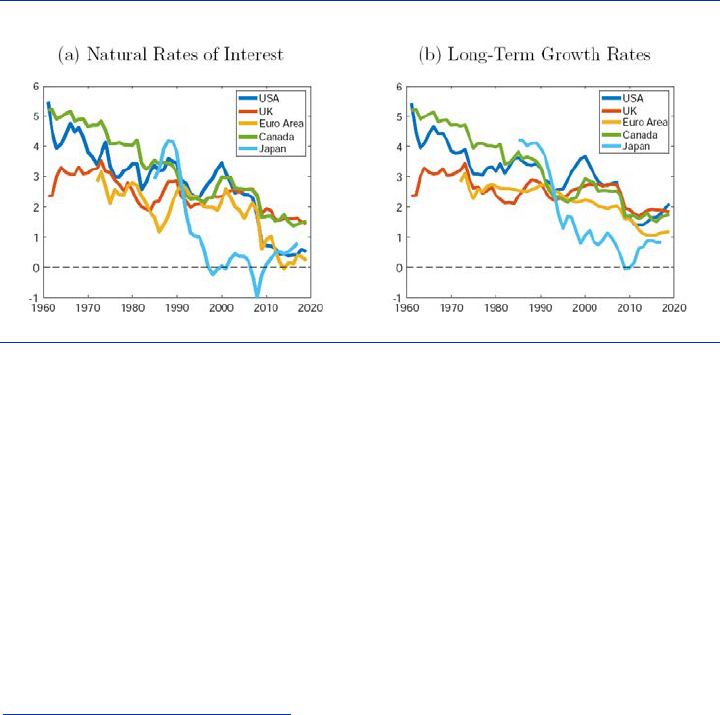
ECB Forum on Central Banking, November 2020
187
level of inflation, the fall in the natural rate implies that nominal rates must fall in
tandem.
Lower average nominal rates mean, however, that the effective lower bound on
nominal interest rates becomes an increasingly relevant constraint for the conduct of
monetary policy.
3
Illustrating this trend, advanced economies have spent increasing
amounts of time in a situation where policy rates are either close to zero or even
negative.
4
Recent experience in advanced economies furthermore illustrates that the inability to
lower nominal rates further is associated with a considerable and rather persistent
undershooting of the inflation target, despite all the newly instituted quantitative
easing policies deployed by central banks. The persistent inflation shortfall risks
unanchoring private-sector inflation expectations, which would have further adverse
consequences for inflation outcomes.
Chart 1
Natural rates and long-term growth rates in advanced economies
(growth rates and interest rates in percentage points)
Sources: Holston et al. (2017), Fujiwara et al. (2016).
Drawing on recent work with a number of co-authors and the monetary policy
literature more generally, the present paper argues that the situation may actually be
even more serious than indicated by the previous arguments. This is so because
advanced economies experienced – in tandem with the decrease in natural rates of
interest – a considerable increase in the volatility of housing prices (Adam, Pfaeuti
and Reinelt (2020)) and equity prices.
Increased asset price volatility further complicates monetary policy for a variety of
reasons. Collateral constraints, for example, may become more easily binding, the
risk of corporate and private defaults may periodically increase, and investment
booms and busts may be triggered by the booms and busts in asset prices.
3
A lower bound exists because investors can always swap bank deposits into zero-interest bearing
cash, which prevents interest rates on bank deposits from falling significantly below zero.
4
In the Euro Area this has been so since 2012; in the United States from the end of 2008 up until the
end of 2015 and then again since the second quarter of 2020; in Japan nominal rates were zero since
1999, with only brief interruptions.

ECB Forum on Central Banking, November 2020
188
Furthermore, evidence on investor expectations obtained from investor surveys
shows that the observed amounts of price volatility in housing and stock markets are
unlikely efficient, instead are at least partly driven by systematic patterns of over-
optimism and over-pessimism (Vissing-Jorgensen (2003), Bacchetta, Mertens and
Wincoop, (2009), Greenwood and Shleifer (2014), Adam, Marcet and Beutel (2017),
Adam, Matveev and Nagel (2020), Adam, Pfaeuti and Reinelt (2020)). And perhaps,
even more worryingly, it is perfectly conceivable that the observed fall in the average
level of the natural rate actually triggered the increased instability in asset markets,
as waves of investor optimism and pessimism become more likely when safe real
interest rates are low (Adam and Merkel (2019)).
To the extent that the observed volatility increase in asset prices fails to be justified
by fundamental factors, it will exacerbate the lower bound problem for monetary
policy. Monetary policy is then not only confronted with lower average nominal rates,
but it also has to vary nominal rates more actively in order to counteract the adverse
effects of increased asset price volatility, e.g., the investment booms associated with
asset price booms. The effective lower bound on nominal rates will thus become an
even more stringent constraint.
5
In light of these observations, the paper summarizes recent academic research and
discusses the implications of lower natural rates and increased asset price volatility
for the conduct of optimal monetary policy when policy faces a lower-bound
constraint on nominal interest rates. It focuses on the implications for (1) the optimal
inflation target and (2) the desirability to ‘lean-against’ asset price movements. The
paper also discusses mechanisms through which asset price volatility rises when
(safe) real interest rates fall.
The quantitative and qualitative implications of lower natural rates and increased
asset price volatility are a function of whether heightened asset price volatility is
considered to be efficient or inefficient, e.g., driven by increased waves of investor
optimism and pessimism.
If increased asset price volatility is judged to be efficient, then the observed fall in
average natural rates justifies only a small increase in the inflation target (Adam,
Pfaeuti and Reinelt (2020)): as the average natural rate falls from around 3% to a
level close to zero, the inflation target optimally increases by less than 0.4%. In
contrast, if the increase in asset price volatility is judged to be inefficient, then a
corresponding fall in the average natural rate justifies a much stronger increase in
the inflation target by around one 1%. This is illustrated in Chart 6 in section 4.1.
The economic force triggering the previous finding is that – in the presence of
subjective investor beliefs – a fall in the average level of the natural rate leads to
higher volatility in the natural rate, in line with the empirical evidence available for
advanced economies. The increased volatility of the natural rate reinforces the
stringency of the lower bound constraint for monetary policy. The optimal policy
5
Adam, Pfaeuti and Reinelt (2020) show how the volatility of the natural rate can increase as its average
level falls and provide evidence that the volatility of the natural rate has increased over time.
ECB Forum on Central Banking, November 2020
189
reaction to these developments is to promise a somewhat higher average inflation
rate.
The optimal response to housing price movements similarly depends on whether or
not asset price volatility is considered to be efficient. With efficient asset prices,
optimal monetary policy can be conducted without reference to housing prices and
monetary policy can focus exclusively on the output gap and inflation (Adam and
Woodford (2020)). Yet, if subjective belief dynamics amplify fundamentally justified
housing price movements, as investor survey data suggests, then monetary policy
should ‘lean-against’ housing price movements, i.e., undershoot its normal targets for
inflation when housing prices rise and overshoot its usual targets when housing
prices fall (Caines and Winkler (2018), Adam and Woodford (2020), Adam, Pfaeuti
and Reinelt (2020)).
The remainder of the paper is structured as follows: Section 2 summarizes the
international evidence on the changing average level of natural rates and the
changing volatility in housing and stock markets in advanced economies. It also
shows how price fluctuations in housing and stock markets co-move with housing
investment and business investment, which suggests that price fluctuations in these
markets have implications for real allocations. Section 3 discusses key economic
mechanisms that allow the linking of asset price volatility to the level of the safe real
interest rate. It also summarizes evidence that shows that investors’ asset price
expectations are inconsistent with the rational expectations assumption, which
strongly suggests that price fluctuations in these markets fail to be fully efficient.
Section 4 discusses the implications of lower natural rates of interest for the optimal
inflation target and the question of whether policy should ‘lean-against’ housing price
movements.
2 Natural rates and asset price volatility: evidence
This section documents how the volatility of housing prices and stock prices has
evolved over time in a number of advanced economies and how volatility changes
correlate with changes in the average level of the natural rate of interest. The section
summarizes results previously presented in Adam, Pfaeuti and Reinelt (2020) and
adds new evidence on the evolution of price volatility in equity markets.
The fluctuations in basic valuation ratios, e.g., the price-to-rent (PR) ratio in housing
markets or the price-to-dividend (PD) ratio in stock markets, are generally large and
very persistent, which makes it difficult to estimate volatility and volatility changes
precisely. To deal with this issue, one has to consider volatility changes across long
periods of time, so as to increase the chances of detecting statistically significant
volatility changes.

ECB Forum on Central Banking, November 2020
190
Chart 2
Standard deviation of valuation ratios in housing and stock markets
Notes: The figure reports the standard deviation of the two valuation ratios. Numbers reported at the bottom are robust p-values
(Newey-West) for the null hypothesis that the standard deviations in the sub-samples are identical. Error bands indicate robust 90%
confidence intervals for the estimated standard deviation. The reported numbers for the price-to-rent ratio differ from the ones in Adam,
Pfaeuti and Reinelt (2020) because they compute the standard deviation in terms of percent deviation from sample mean. The latter
leads to very similar conclusions.
Chart 2 depicts the standard deviation of the PR-ratio and of the PD-ratio, comparing
the 30-year period 1960-1989 to the subsequent 30-year period 1990-2019.
6
Panel
(a) shows that the point estimate for the standard deviation of the PR-ratio has
increased in all considered economies. The increase in the point estimate is
quantitatively large and statistically significant at the 10% level in 4 of the 6
considered countries.
7
Panel (b) in Chart 2 depicts the standard deviation of the PD ratio across the two
sample periods. While the point estimate has increased in 4 of the 6 countries, the
increase is statistically significant at the 10% level only in the United States, and
marginally so for Canada. The volatility reductions in Japan and France are both
insignificant.
8
The insignificant result for Japan is perhaps not too surprising, given
that the sample split occurs close to peak of the Japanese stock market boom in the
late 1980s, causing the run-up to be part of the pre-1990 sample and the subsequent
bust to be part of the post-1990 sample.
9
Overall, Chart 2 provides strong evidence in favour of an increase in the volatility of
housing prices and somewhat weaker evidence in favour of an increase in stock
price volatility.
Chart 3 shows how the change in the average natural rate (pre- vs. post-1990, on
the x-axis) compares with the change in asset price volatility (pre- vs. post-1990, on
6
For housing markets, the PR-ratio is generally available only back to 1970. We take the series as far
back as they are available.
7
Importantly, this conclusion is not driven by the fact that PR-ratios were on average larger in the second
half of the sample period. Considering instead the percent deviation of the PR-ratio from its period-
specific mean leads to very similar results.
8
The volatility of the Japanese stock market is so large because it experienced in around 1990 one of
advanced economies’ largest stock price boom-bust episodes (in terms of the PD-ratio).
9
Given that the natural rate declined significantly earlier in Japan, see Chart 1, one might argue that the
Japanese sample should be split well before 1990 to be comparable with the other advanced
economies.
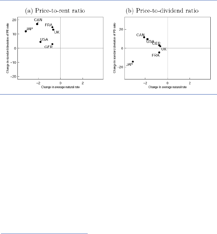
ECB Forum on Central Banking, November 2020
191
the y-axis). Panel (a) depicts the volatility change of the PR-ratio and Panel (b) the
volatility change of the PD-ratio.
Panel (a) shows that all countries are located in the upper-left quadrant, i.e., housing
price volatility increased and natural rates fell in all countries. Moreover, there is a
clear negative relationship between the changes in the average natural rate and the
changes in housing price volatility, illustrating that countries that experienced larger
drops in the natural rate also experienced larger increase in housing price volatility.
A similar pattern can be observed in Panel (b) of Chart 3, which considers changes
in stock price volatility and average natural rates. Most countries lie in the upper-left
quadrant. Moreover, abstracting from Japan, which is an outlier for reasons
discussed before, there is also a near-perfect negative relationship between changes
in the average natural rate and changes in the volatility of the PD-ratio.
Chart 3
Change in average natural rates vs. change in std. deviation of valuation ratios (pre-
1990 vs. post-1990)
Notes: The change in the average natural rate is based on the natural rate estimates of Holston et al. (2017) and Fujiwara et al (2016).
The change of the standard deviations of the PR-ratio and PD-ratio is from Chart 2.
The previous evidence is consistent with the notion that lower natural rates may
have caused the observed volatility increase in housing and stock markets.
10
Yet, an
important open question is to what extent increased asset price movements matter
for real allocations. This question is particularly pressing because it has been argued
in the past that the stock market, for instance, is a sideshow when it comes to
business investment (Morck, Shleifer, Vishny (1990)). While more recent empirical
evidence has been more supportive of the notion that investment at the firm level
depends on the firm’s stock market price, e.g., Baker, Stein and Wurgler (2003),
Chart 4 presents evidence for the aggregate economy.
10
This holds true despite the fact that the presented empirical evidence does not identify any causal
relationship.

ECB Forum on Central Banking, November 2020
192
Chart 4
Correlation between valuation ratios and investment rates
Notes: The figure reports the correlation between the valuation ratios and the linearly detrended investment-to-GDP ratios. Error bands
indicate robust 90% confidence intervals (Newey-West) and have been computed using the delta method. Panel (a) is from Adam,
Pfaeuti and Reinelt (2020).
Panel (a) in Chart 4 reports the correlation (pre- and post-1990) between the PR-
ratio and the ratio of housing investment to GDP. It shows that all point estimates,
except for one, are positive and that 9 out of the 12 reported correlations are
significant at the 10% level. In many cases, the correlations are also pretty large.
This suggests that high housing prices trigger high housing investment, so that
housing price fluctuations matter for real allocations.
11
Panel (b) in Chart 4 depicts the correlation (pre-/post-1990) between the PR-ratio
and the ratio of investment into equipment to GDP.
12
The point estimates for all
correlations turn out to be positive and most of them are quantitatively large. Of the
reported 11 correlations, 8 are statistically significant at the 10% level. This again
suggests that high stock prices trigger high business investment, so that stock price
fluctuations matter for real allocations.
3 Economic mechanisms linking growth rates, real interest
rates and asset price volatility
A number of economic mechanisms can explain why lower growth rates are
associated with lower levels of real interest rates and increased asset price volatility.
To make a sharp distinction, this section focuses on a frictionless efficient market
model, which serves as a useful theoretical benchmark. It then considers pricing
setups that allow for a role of speculative price expectations in asset pricing. The
latter is motivated by survey evidence on investor expectations, which shows that
11
Again, the evidence presented in Chart 4 does not identify a causal relationship.
12
Since this investment series is not available for the U.K. prior to 1990, we report only post-1990
correlations for the U.K.

ECB Forum on Central Banking, November 2020
193
subjectively expected prices deviate in systematic ways from the behaviour of
realized prices.
13
While both setups provide mechanisms through which low safe interest rates
increase asset price volatility, they differ with regard to the welfare implications of
increased asset price volatility. Under the efficient market model, increased asset
price volatility has, per se, no welfare consequences. With speculative expectations,
this fails to be true, which in turn will explain why the two setups give rise to rather
different implications for the optimal inflation target and the desirability to lean-
against asset price movements.
Clearly, the distinction between efficient and inefficient fluctuations in asset prices
emphasized in this section does not exclude that an increase in the efficient
fluctuations of asset prices alone can already have negative welfare implications.
This can be the case in the presence of additional frictions, e.g., borrowing/collateral
constraints or commitment problems that give rise to default incentives. For
simplicity, the subsequent discussion abstracts from these additional frictions.
3.1 Average growth rates, real interest rates and natural rates
Both considered setups rely on the same fundamental pricing equation for the safe
real interest rate
. This equation will allow drawing a connection between the
economy’s average growth rate and the average safe real interest rate. The latter
can furthermore be related to the average natural rate.
The fundamental asset pricing equation for a safe real short-term asset is
(1 +
)
[
,
] = 1,
where 0 < < 1 denotes the time discount factor, which indicates how strongly
agents discount the future (lower values indicated higher impatience) and
[
,
]
denotes the expected growth rate of the marginal utility of consumption, which is
inversely related to economic growth, as higher growth means that the marginal unit
of consumption tomorrow generates less additional utility. Expectations are based
either on rational or subjective beliefs.
14
Taking unconditional (rational) expectations of the previous equation, one obtains an
expression characterizing the economy’s average safe real interest rate r.
15
:
(1 + r)E[
,
] = 1
13
Low real interest rates can affect asset price volatility through additional channels considered by neither
of these setups. For instance, lower real rates provide investors with better financing conditions, which
may make leveraged positions in asset markets more attractive and thereby increase market instability.
14
The expectation is formed in period t and is for the inverse of the growth rate of marginal utility between
periods t and t+1.
15
The expression holds independently of whether beliefs are rational or not, as long as subjective
expectations are on average unbiased. To simplify notation, it uses the approximation
,
E
,
.

ECB Forum on Central Banking, November 2020
194
The average safe interest rate r is a function of the time discount factor and the
objective average of the growth rate of marginal utility
,
.
When investors become more patient, i.e., as the time discount factor moves
closer to one, the safe interest rate r must fall for the previous equation to continue
to hold. Likewise, as the average growth rate of the economy slows down, the
average growth rate of marginal utility rises. With E
,
rising, the real safe
interest rate r must fall. The pricing equation is thus consistent with the empirical
observation that lower average growth rates in advanced economies have been
accompanied by a fall in average safe real interest rates.
Many economic models furthermore imply that the average safe real interest rate is
equal to the average natural rate of interest, whenever the environment is
characterized by stable inflation. To see why this is the case, assume – for the
purpose of reaching a contradiction – that real interest rates were set permanently
below (above) the average safe real rate, as determined by the previous equation.
The demand stimulation (strangulation) associated with such real interest rate
policies would cause the output gap to become ever more positive (negative). This,
however, would be in consistent with stable inflation in the presence of a Phillips
curve relationship. In a stationary environment without runaway inflation or deflation,
the average natural rate is thus equal to the average real interest rate.
3.2 The Efficient Markets view
Under the efficient market model, the fundamental asset pricing equation for a risky
asset (housing/equities) is given by
p
=
+
E
[
p
]
(1)
where p
denotes the asset price
16
and
the current-period payoff of the asset,
which consist of dividends in the case of stocks and rents or rental utility in the case
of housing.
17
If investors hold rational expectations, one can iterate forward on the previous
equation
18
and express the asset price as the expected discounted present value of
future payoffs:
p
= E
(1 + )
.
16
To simplify notation and make the argument more transparent, the asset price is expressed here in
marginal utility units, with marginal utility being detrended by the steady state growth rate of marginal
utility.
17
Rent payouts are equally expressed in marginal utility units.
18
Adam and Marcet (2011) and Adam, Marcet and Beutel (2017) explain why such forward-iteration does
generally not follow from individual rationality, instead provides agents with market-knowledge (rational
expectations).

ECB Forum on Central Banking, November 2020
195
The price-to-rent/price-to-dividend ratio is given by p
/
and will be more variable
when the safe interest rate is lower: since future payoffs get discounted less, the
asset price ratio p
/
will move more (in percentage terms) in response to any given
movement in the current payoff
. 111F
19
While the asset price ratio becomes more variable as the average safe average
interest falls, increased asset price volatility is efficient and thus is not a source of
concern for monetary policy. Clearly, this conclusion hinges on the assumption that
investors’ expectations about future asset prices are rational. (It also hinges on the
absence of other frictions in the economy). As discussed in the next section, there is
mounting empirical evidence showing that rationality of expectations fails to hold.
3.3 Speculative elements in asset price expectations
A growing body of research in asset pricing has examined survey data on investor
expectations. This literature finds that the time-series dynamics of investors’
return/capital gain expectations are in conflict with the actual behaviour of
returns/capital gains. In particular, expected returns/capital gains display (1) different
cyclicality than actual return/capital gains, and (2) investor expectations about the
future level of housing and stock prices display too much sluggishness in their
adjustments. These two points are discussed in the following subsections.
3.3.1 Cyclicality of actual versus expected returns/capital gains
While future stock returns and capital gains are counter-cyclical, i.e., tend to be low
(high) when the price-dividend ratio is high (low), the survey evidence shows that
investors’ return and capital gain expectations are pro-cyclical: subjective expected
returns/capital gains are high (low) in times of high (low) price-dividend ratios
(Vissing-Jorgensen(2003), Bacchetta et al. (2009), Greenwood and Shleifer (2014),
and Adam, Marcet and Beutel (2017), Adam, Matveev and Nagel (2020)).
The different cyclicality of realized and expected stock returns/capital gains is
illustrated in table 1 using results from Adam, Marcet and Beutel (2017). The table
reports the regression coefficients and of the following two regressions
,
= +
+
(2)
[
,
] = +
+
(3)
where
,
denotes the realized stock return (or capital gain) between period and
+ ,
[
,
] the survey expectation of the corresponding stock return (or capital
gain) as of period , and
/
the price-dividend (PD) ratio in period .
20
19
This assumes that the process for
follows a stationary auto-regressive process, see Lemma 1 in
Adam, Pfaeuti and Reinelt (2020) for details.
20
The residuals (
,
) are potentially serially correlated.

ECB Forum on Central Banking, November 2020
196
Table 1
The different cyclicality of realized and expected returns/capital gains in stock
markets
Source: Table 1A from Adam, Marcet and Beutel (2017).
Notes: The columns labelled ĉ report the estimate of the coefficient c in equation (2). The columns labelled ĉ report the estimate of the
coefficient c in equation (3). The columns labelled bias report the small sample bias correction and the columns labelled p-value report
the small sample bias-corrected p-value for the null hypothesis that c=c. The leftmost column indicates the survey sources (UBS
Survey, Chief Financial Officer Survey and Robert Shiller’s investor survey), the horizon of the forecast (1 year, 10 years), the way real
returns have been computed (inflation expectations from the Survey of Professional Forecasters (SPF), inflation expectations from the
Michigan Survey), and various wealth categories (all: all investors in the survey, >100k: only investors with more than 100k USD in
financial wealth).
Table 1 reports the estimates of the coefficients and for various survey sources,
various survey subsamples and various forecast horizons.
21
It performs the analysis
once using the survey mean and once using the survey median, to account for
potential outliers. It shows that the coefficient for realized returns is always
negative: future realized returns/capital gains are low (high) when the price-dividend
ratio is high (low), i.e., actual returns/capital gains are counter-cyclical. In contrast,
the estimated coefficient for expected returns is always positive: expected
returns/capital gains are high (low) when the PD is high (low), i.e., expected returns
are pro-cyclical. The table also tests the hypothesis that both coefficients are equal.
This test takes in to account potential small-sample bias corrections (also reported in
Table 1) that may arise from the fact that the predictor variable (the PD-ratio) is
serially correlated (Stambaugh(1999)). In all cases, equality of the regression
coefficients is rejected at the 5% significance level and in the vast majority of cases
the rejection is significant at the 1% level.
It turns out that the empirical findings for actual and expected capital gains in stock
markets proves to be rather robust and can also be found for housing market
expectations. Table 2 reports the regression coefficients and of the following two
regressions
,
= +
+
(4)
[
,
] = +
+
, (5)
21
See the explanatory notes below the table for a detailed description. Table 1 uses real returns and
capital gains (realized and expected), but results are robust to using nominal returns/capital gains
instead.

ECB Forum on Central Banking, November 2020
197
where
,
denotes the realized housing capital gain between period and period
+ 1,
[
,
] the corresponding survey expectations of the capital gain from the
Michigan survey, which covers the years 2007-2019, and
/
the price-to-rent (PR)
ratio in period .
22
Table 2 shows that future capital gains in housing markets are negatively associated
with the PR-ratio, i.e., are counter-cyclical. In contrast, survey expectations of future
capital gains are positively associated with the PR-ratio, i.e., are pro-cyclical. This
difference is highly statistically significant for the survey average and significant at
approximately the 5% level for the survey median, again accounting for potential
small-sample biases in estimation.
Overall, table 2 suggests that expectations about capital gains in housing markets
show the same puzzling property as survey expectations in stock markets.
Table 2
The different cyclicality of realized and expected capital gains in housing markets
Source: Adam, Pfaeuti and Reinelt (2020)
Notes: The columns labelled ĉ report the estimate of the coefficient c in equation (4) using the Case-Shiller home price index for the
United States. The columns labelled ĉ report the estimate of the coefficient c in equation (4) using the Michigan survey. The columns
labelled bias report the small sample bias correction, performed as in Table1A in Adam, Marcet and Beutel (2017), and the columns
labelled p-value report the small sample bias-corrected p-value for the null hypothesis that c=c.
3.3.2 Sluggish adjustment of housing and stock price expectations
This section presents evidence for the fact that expectations about the level of future
housing and stock prices adjust sluggishly. In particular, past upward revisions in
investor expectations predict that future outcomes will on average exceed the
upwardly-revised expectations. As a result, past forecast revisions predict future
forecast errors in the same direction, which is inconsistent with forecasts being
rational.
Following Coibion and Gorodnichenko (2015), one can consider regressions of the
form
= +
+
, (6)
where
denotes the housing or stock price in period + and
the survey
forecast of this price as of period . The expression on the left-hand side of equation
22
The residuals (
,
) are potentially serially correlated.
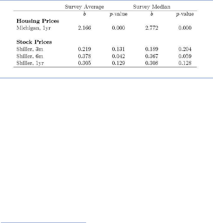
ECB Forum on Central Banking, November 2020
198
(6) is the forecast error about the level of the future housing/stock price. The right-
hand side of the equation uses the belief revision about -period ahead
stock/housing prices between periods 1 and . Under the assumption of rational
expectations, past forecast revisions should not predict future forecast errors at any
forecast horizon : past forecast are part of agents’ information set and that
information should be contained in any rational forecast. Under the hypothesis of
rational expectations, one should thus find = 0.
Table 3 shows, however, that one obtains > 0 in all cases.
23
The evidence is highly
statistically significant for housing price expectations, but less significant for stock
markets. Overall, however, results all point in the same direction: past revisions of
expectations in a certain direction predict further forecast errors in the same
direction, i.e., the belief revisions are insufficiently strong. Expectations are thus
adjusted sluggishly over time.
Table 3
Sluggish adjustment of expected housing and stock prices (levels)
Source: Adam, Pfaeuti and Reinelt (2020).
Notes: The first column indicates the survey sources (Michigan, Shiller), the forecast horizons (3 months, 6 months, 1 year) and the
predicted variable (housing price, stock price). The columns labelled b report the estimate of the coefficient b in equation (6). The
reported p-values are robust (Newey-West with 4 lags).
3.4 Asset price volatility with speculative beliefs and the effects of low
real interest rates
This section explores the asset pricing implications of falling real interest rates when
subjective capital gain expectations feature pro-cyclical fluctuations and sluggish
updating, in line with the empirical evidence provided in the previous sections. This
section is based on a strongly simplified setup of Adam and Merkel (2019), who
consider a fully-fledged business cycle model. The goal here is to explain in simple
terms how low real interest rates increase asset price fluctuations.
Let
denote investors’ subjective capital expectations
24
=
[
/
]
.
23
Table 3 only uses surveys that ask for investors’ capital gain expectations. Surveys that report return
expectations require imputing expected dividends, to be able to compute a level forecast of the asset
price.
24
Capital gain expectations should be interpreted again in marginal-utility adjusted terms.

ECB Forum on Central Banking, November 2020
199
Given these expectations, the fundamental asset pricing equation (1) delivers the
equilibrium asset price
p
=
/()
, (7)
which depends positively on the current payoff
and positively on the subjective
capital gain expectations
.
25
Equation (7) shows how high (low) capital gain expectations give rise to a high (low)
asset price and a high price-to-dividend or price-to-rent ratio (p
/
). In line with the
evidence documented in the previous sections, subjective capital gain beliefs will
thus necessarily be pro-cyclical, even if realized capital gains are counter-cyclical.
To understand the dynamics of asset prices, one needs to take a stand on how
subjective capital gain beliefs are adjusted over time. It makes sense to consider an
empirically plausible belief specification that is consistent with the evidence on
sluggish adjustment and that gives rise to counter-cyclical realized capital gains.
Adam, Marcet and Nicolini (2016) show optimal (Bayesian) belief updating by
investors can give rise to an updating equation of the form
=
+
(
/
)
, (8)
where the parameter 1/ (the Kalman gain) determines how strongly capital gain
beliefs
get adjusted in light of the observed capital gain surprise (
/
).
26
Importantly, if 1/ is sufficiently small, then these subjective beliefs will display
sluggish adjustment in line with the empirical evidence (Adam, Pfaeuti and Reinelt
(2020)). And as shown in the next section, realized capital gains will be counter-
cyclical, in line with the data.
3.4.1 Belief-driven boom-bust dynamics in asset prices
Belief updating equation (8) and asset price equation (7) jointly imply that belief
changes and price realizations can mutually reinforce each other in a way that
generates persistent boom-bust cycles in asset prices (Adam, Marcet and Nicolini
(2016)). These cycles will drive the counter-cyclicality of realized returns.
To understand why this is the case, consider a situation in which the current payout
happens to be unusually large. From equation (7) it follows that – for given capital
gain expectations
– the realized asset price and thus the realized capital gain
/
will be unusually large. Given the belief updating equation (8) this implies
that future capital beliefs
will be pushed upwards. The upward revision in beliefs
produces –according to equation (7) – further capital gains in the next period. There
is thus the possibility of a persistent asset price boom where prices and investor
25
As explained in Adam and Marcet (2011), beliefs about the present value of dividends are irrelevant for
asset pricing in the presence of subjective price beliefs, see also Adam, Marcet and Beutel (2017).
26
One has to additionally impose an upper bound on the beliefs to ensure
< 1 + , so that prices
remain well-defined in equation (7).
ECB Forum on Central Banking, November 2020
200
optimism rise together: upward revisions in beliefs produce capital gains and capital
gains produce further upward belief revisions.
The boom will come to an end once the realized capital gains start to fall short of
investors’ high capital expectations. At this point, there will be a Minsky moment:
capital gain expectations are high but get revised downwards (equation (8)); the
downward revision produces capital losses (equation (7)) and further downward
revision in beliefs. Asset prices will then fall and can even persistently undershoot
their efficient market value. The mean-reversion of asset prices implies that realized
returns/capital gains will indeed be counter-cyclical, even though expected returns
are pro-cyclical, in line with the empirical evidence.
Since these boom-bust like movements in asset prices will not be efficient they will
have the potential to distort the efficient investment decision, as suggested by the
evidence in Chart 4, and thus have adverse welfare implications.
In the context of housing price dynamics, for example, a housing price boom that is
fuelled by increased investor optimism is likely going to lead to an overaccumulation
of the housing stock, in line with what has been observed in some countries during
the run-up to the 2007 financial crisis (Adam, Marcet and Kuang (2012), Kaplan,
Mitman and Violante (2020)). Likewise, a stock price boom, e.g., one created by the
arrival of new optimistic narratives, has been shown to lead to investment booms,
especially in equity-dependent firms (Baker, Stein and Wurgler (2003)), see also
Gilchrist et al. (2005)).
Obviously, boom-bust cycles in asset prices can have adverse welfare implications
via a number of other economic channels, e.g., by redistributing wealth between
different investors (Nagel and Greenwood (2009), Adam, Beutel, Marcet and Merkel
(2015)).
3.4.2 The effect of low safe real rates on boom-bust dynamics
This section explains how belief-driven boom-bust cycles, as described in the
previous section, become more likely as the safe real interest rate falls. The fact
that this is the case suggests that the observed increase in asset price volatility is
actually a by-product of the observed fall in the safe real interest rate.
As in the previous section, consider a fundamental impulse from an unusually high
payout
. The capital gain produced by the positive fundamental will increase
current capital gains and thereby the capital gain expectations
in the next
period. Yet, for any given increase in capital gain expectations
, the capital gains
in period t+1 will be larger the lower the safe rate , see equation (7). Asset prices
thus become more sensitive to belief revisions when real interest rates are low.
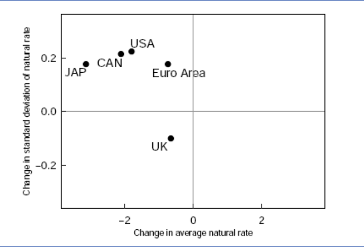
ECB Forum on Central Banking, November 2020
201
Chart 5
Change in average natural rate vs. change in std. deviation of natural rate
(pre-1990 vs. post-1990)
Source: Adam, Pfaeuti and Reinelt (2020).
Notes: The change in the average natural rate is based on the natural rate estimates of Holston et al. (2017) and Fujiwara et al (2016).
The standard deviation of the natural rate has been computed by linearly detrending the natural rate to take into account its time trend.
Given this, the chances of any initial fundamental impulse to generate a self-
sustaining increase in beliefs and asset prices become higher. Adam and Merkel
(2019) illustrate this mechanism in detail, showing how – when real interest rates are
low – smaller-sized shocks or a smaller number of shocks of any given size can
generate self-sustaining boom-bust dynamics.
The prediction that boom-bust cycles become more frequent as interest rates fall is
in line with the repeated housing and stock price cycles experienced in advanced
economies since the 1990’s.
3.4.3 Boom-bust dynamics and the volatility of the natural rate
To the extent that the fall in the safe real interest rates generates an increase in
(socially inefficient) asset price boom-bust cycles and to the extent that these price
cycles are accompanied by corresponding cycles in investment (see Chart 4),
lending, corporate and household defaults, etc., the increased occurrence of price
cycles will have implications for the volatility of the natural rate.
The volatility of the natural rate is affected because stabilizing inflation in such an
environment will require that monetary policy counteracts some of the covariates of
boom-bust cycles, e.g., the associated investment cycles (Adam, Pfaeuti and Reinelt
(2020)). Interestingly, the empirical evidence suggests that the decrease in the
average natural rate has in fact been accompanied by an increase in the volatility of
natural rates.

ECB Forum on Central Banking, November 2020
202
This is illustrated in Chart 5, which compares the change in the average natural rate
(pre-/post-1990) on the x-axis to the change in the volatility of natural rate (pre-/post-
1990) on the y-axis. For all considered currency areas, except for the U.K., the
decrease in the average natural rates was associated with an increase in the
volatility of the natural rate. This suggests that lower average natural rates may in
fact have contributed to an increase in the volatility of the natural rate.
4 Monetary policy implications of lower natural rates
This section discusses the implications lower average natural rates and increased
housing price volatility have for (1) the level of the optimal inflation target and for (2)
the conduct of monetary policy in response to housing sector disturbances. As will
become clear, the monetary policy conclusions depend in crucial ways on the
economic drivers of increased asset price volatility (Adam and Woodford (2020),
Adam, Pfaeuti and Reinelt (2020)).
4.1 Implications for the optimal inflation target
We start by considering the case in which the empirically observed increase in asset
price volatility is judged to be efficient, as would be the case under the conditions
outlined in section 3.2. While the empirical evidence provided in section 3.3 does not
support the interpretation that asset price fluctuations are efficient, the efficient
market setting nevertheless provides an important reference point that allows for a
better understanding of the additional implications generated by inefficient
fluctuations in asset prices.
With efficient asset price fluctuations, lower average natural interest rates will
depress the average nominal interest rates (taking the inflation target as given).
Lower nominal rates, however, cause the effective lower bound constraint on
nominal rates to become increasingly binding. One can thus ask the question
whether and to what extent the presence of a lower bound constraint justifies
increasing the inflation target and to what extent this increase depends on the
average level of the natural rate.
The intuition for why the inflation target optimally increases when policy is
constrained by the lower bound on nominal rates is rather simple: since real interest
rates cannot be lowered further via a reduction in nominal rates, the only other tool
available for lowering real interest rates is a promise to achieve higher future inflation
in the future.
27
Such promises of higher future inflation, which are part of the optimal
conduct of monetary policy when policy is constrained by the lower bound, increase
the average inflation rate.
27
This is so because the real rate is the nominal rate minus the expected inflation rate. The argument
implicitly assumes that the promises, to the extent that they are feasible, are correctly anticipated by
the private sector.

ECB Forum on Central Banking, November 2020
203
Chart 6
Optimal increase of the inflation target due to the effective lower bound on nominal
rates
Source: Adam, Pfaeuti and Reinelt (2020).
Chart 6 reports the optimal inflation target, i.e., the average inflation outcome under
optimal conduct of monetary policy. For each considered level of the average natural
rate (on the x-axis), the chart reports the optimal inflation target (on the y-axis) in an
economy with an effective lower bound constraint, relative to the target that would be
optimal in the absence of a lower-bound constraint.
28
Chart 6 illustrates that the presence of the lower bound constraint justifies targeting
higher average inflation and that this effect is stronger, the lower the average natural
interest rate. The quantitative effect of the lower-bound constraint on the inflation
target is, however, relatively muted when asset prices are efficient. Even with
average natural rates dropping permanently from a level of 3.3% to a level of 0.125%
per year, the inflation target increases by less than 0.4%.
This result differs strongly from the findings reported in Andrade et al. (2019), who
find a near one-to-one relationship between drops in the average natural rate and
the optimal inflation target. The source of this difference is that Chart 6 considers
fully optimal monetary stabilization policy while Andrade et al. consider Taylor-type
monetary policies and optimize only with respect to the intercept term in the Taylor
rule.
28
Chart 6 is based on a calibrated workhorse New Keynesian sticky price model featuring also a housing
sector, see Adam, Pfaeuti, Reinelt (2020) for details. In the absence of a lower bound constraint, the
optimal inflation target is zero, because the model abstracts from other forces that make targeting
positive average rates of inflation optimal, e.g., the ones considered in Adam and Weber (2019, 2020).
0 0.5 1 1.5 2 2.5 3 3.5 4
0
0.2
0.4
0.6
0.8
1
1.2
1.4
1.6
1.8
2

ECB Forum on Central Banking, November 2020
204
Chart 6 also reports the optimal increase in the inflation target for the case where
housing prices are driven – at least partly – by fluctuations in subjective housing
price expectations, in line with the empirical evidence from section 3.3. The reported
inflation target increase now comprises the combined effect of a lower bound and of
fluctuations of subjective housing price expectations.
Two findings are remarkable. First, the combined effect of subjective beliefs and a
lower bound constraint is always larger than the effect of the lower bound constraint
alone, i.e., both effects work in the same direction. Second, as the average natural
rate falls, the optimal inflation target increases much more strongly in the setting with
subjective housing beliefs.
The reason for the latter finding is that lower natural real rates of interest not only put
downward pressure on nominal rates, but also increase the likelihood of boom-bust
cycles in asset prices, as discussed in section 3.4.3. These boom-bust cycles make
the natural rate more volatile, in line with the evidence shown in Chart 5, and thereby
increase the likelihood of hitting the lower bound, unless policy adjusts by increasing
the inflation target.
The combined effect of a lower average level of the natural rate and of increased
natural rate volatility justifies a stronger increase in the optimal inflation target as the
natural rates fall: instead of increasing by less than 0.4% when the natural rate falls
from 3.3% to 0.125%, as was the case with efficient asset prices, the inflation target
now increases by a full 1%. This shows how the fall in average natural rates can
rationalize a significant increase in the optimal inflation target.
4.2 Implications for the policy response to asset price booms/busts
This section discusses some of the factors affecting the optimal monetary policy
response to increased asset price movements. As with the inflation target, the
optimal policy response turns out to depend crucially on the economic forces driving
the increase in asset price volatility.
If the observed increase in asset price volatility is judged to be efficient, e.g., reflects
only the decrease in the safe real interest rate, as discussed in section 3.2, then in
the absence of other frictions (besides pricing frictions), increased asset price
volatility will not be relevant for the stabilization goals of welfare-oriented monetary
policy. In particular, there is no need for monetary policy to respond to asset price
movements (Adam and Woodford (2020)).
29
In light of the empirical evidence discussed in section 3.3, however, it is unlikely that
asset price fluctuations are entirely efficient, as investors’ asset price expectations
fail to be fully rational. In fact, the dynamics of the empirically observed subjective
capital gain expectations suggests that movements in subjective capital gain
expectations amplify fundamentally justified asset movements and thereby generate
29
As discussed before, the presence of other frictions, e.g., collateral or borrowing constraints, would
overturn this result.
ECB Forum on Central Banking, November 2020
205
excessive asset price volatility (Adam, Marcet, Beutel (2017)). And as discussed in
section 3.4, inefficient asset price volatility increases as the average natural interest
falls (Adam and Merkel (2019)).
To the extent that excessive price volatility has welfare costs, it becomes optimal for
policy to counteract these and the urgency to do so rises as the misalignments
increase in size or frequency. Generally, it would be desirable to have additional
(non-monetary) policy tools available to deal with excessive asset price movements.
While such tools may be deployed in practice, e.g., via time-varying borrowing
restrictions or capital requirements, their effects are likely going to be imperfect,
especially given the fact that the macro-prudential framework in the Euro Area is still
quite imperfect (e.g., covers only banks).
In light of this situation, monetary policy will have to take a decision on how to
respond to any residual asset price movements not addressed by macro-prudential
policies or other policy tools. This is particularly true because monetary policy as a
financial stability tool has the advantage that it “gets in all of the cracks” of the
financial system (Stein (2013)).
The literature has shown that in the presence of subjective belief fluctuations, it can
become optimal for monetary policy to “lean-against” asset price movements. This
holds true for a range of alternative subjective belief specifications (Caines and
Winkler (2018), Adam and Woodford (2020), Adam, Pfaeuti and Reinelt (2020)).
Counteracting asset price movements does thereby not require that monetary policy
properly diagnoses any misalignments in asset prices. Instead, it can be sufficient to
simply react to asset price surprises (Adam and Woodford (2020)) or it can be
approximately optimal to respond to observed capital gains (Caines and Winkler
(2018).
Chart 7, which is based on Adam, Pfaeuti and Reinelt (2020), illustrates the optimal
policy response following a persistent housing demand shock in a setting where
investors extrapolate past housing price increases.
The responses to a positive housing demand shock are shown in blue in Chart 7.
The housing demand shock itself is thereby shown in the upper left panel: housing
demand increases on impact and gradually reverts over time. Following the initial
demand shock, housing prices rise, because housing supply is fixed in the short-
term. The fundamentally justified initial increase in housing prices, however, gets
amplified over time (upper middle panel in Chart 7): in light of the initial capital gains,
investors become somewhat more optimistic about future capital gains (upper right
panel in Chart 7), which drives up housing prices further and generates further
increases in optimism. As a result, housing prices increase for a number of periods,
before slowly reverting direction. This belief-based amplification of housing price
movements illustrates how housing prices can persistently overshoot their efficient
level, which sets in motion an inefficient housing investment boom (and likely a
number of additional distortions). The overinvestment in housing explains the
positive output gap in the lower left panel of Chart 7. To counteract the housing
boom, it becomes optimal for monetary policy to ‘lean-against’ the housing price
ECB Forum on Central Banking, November 2020
206
increase (lower right panel in Chart 7). This causes inflation to temporarily
undershoot it usual target (lower middle panel in Chart 7).
Chart 7
Optimal monetary policy leans against housing prices when housing prices are partly
driven by subjective capital gain optimism
Source: Adam, Pfaeuti and Reinelt (2020).
Chart 7 also highlights that the opposite policy response is optimal when faced
instead with a negative housing demand shock (red coloured lines in the chart).
Policy then persistently lowers nominal interest rates and inflation persistently
overshoots its usual targets by a small amount. The policy response to positive and
negative shocks fails to be entirely symmetric because the presence of a lower
bound constraint on nominal rates has implications for stabilization policy well before
the lower bound constraint is reached (Adam and Billi (2006)).
The results discussed above differ from the conclusions reached in earlier literature,
which focused on rational asset price bubbles. Bernanke and Gertler (1999, 2001),
for example, argue that asset prices do not merit any special role in determining
monetary policy, whenever the central bank takes demand pressures into account.
While this may be true for a setting in which asset prices have demand effects only,
e.g., where asset prices relax collateral constraints, it fails to hold in a setting where
asset price misalignments also give rise to supply distortions (Adam and Woodford
(2020)).
Galì (2014) also considers rational asset price bubbles and argues that monetary
policy may increase the growth rate of (rational) bubbles by raising interest rates in
response to a bubble. Miao, Shen and Wang (2019) show, however, that the
conclusions in Gali (2014) are sensitive to what is assumed about the nature of the
rational bubble process. Moreover, the notion of a rational bubble is not consistent
with the survey evidence presented in section 3.3.
0 4 8 12 16 20
-5
0
5
0 4 8 12 16 20
-10
-5
0
5
10
0 4 8 12 16 20
0.998
0.999
1
1.001
1.002
0 4 8 12 16 20
-0.6
-0.4
-0.2
0
0.2
0.4
0 4 8 12 16 20
-0.1
-0.05
0
0.05
0.1
0 6 12 18
-1
-0.5
0
0.5
1
ECB Forum on Central Banking, November 2020
207
5 Conclusions
Falling natural rates and rising asset price volatility pose important challenges for
monetary policymakers in advanced economies, which are increasingly constrained
by the effective lower bound on monetary policy.
The paper argues that the fall in natural rates justifies an increase in the optimal
inflation target. The extent of the increase depends on how one interprets the
observed increase in asset price volatility. If the increase is not due to efficient
forces, then the increase in the inflation target should be more pronounced and
monetary policy should lean against asset price movements.
What if falling long-term growth rates have caused the fall in natural rates and the
increase in asset price volatility, as many economic models suggest? Then an even
better policy response – albeit one beyond the realm of monetary policy – consists of
enacting structural policies that contribute to raising advanced economies’ growth
potential. Such policies would also simplify the task of monetary policy.
References
Adam, K, Beutel, J., Marcet, A. and Merkel, S. (2015), “Can a Financial Transaction
Tax Prevent Stock Price Booms?”, Journal of Monetary Economics, 76, S90-S109.
Adam, K. and Billi, R. (2006), “Optimal Monetary Policy under Commitment with a
Zero Bound on Nominal Interest Rates”, Journal of Money, Credit and Banking, Vol.
38(7),1877-1905.
Adam, K. and Marcet, A. (2011), “Internal Rationality, Imperfect Market Knowledge
and Asset Prices", Journal of Economic Theory, 146, 1224-1252.
Adam, K., Marcet, A. and Beutel, J., (2017), “Stock Price Booms and Expected
Capital Gains”, American Economic Review, 107, 2352–2408.
Adam, K, Matveev, D, and Nagel, S. (2020), “Do Survey Expectations of Stock
Returns Reflect Risk Adjustments?”, Journal of Monetary Economics (forthcoming).
Adam, K., Marcet, A. and Nicolini, J. P., (2016), “Stock Market Volatility and
Learning", Journal of Finance, 71, 33-82.
Adam, K., Marcet. A. and Kuang, P. (2012), “House Price Booms and the Current
Account”, in Acemoglu, D. and Woodford, M. (eds.), NBER Macroeconomics Annual
2011, Volume 26, 77-122, MIT Press.
Adam, K. and Merkel, S. (2019), “Stock Price Cycles and Business Cycles”, ECB
Discussion Paper, No. 2316.
Adam, K., Pfaeuti, O. and Reinelt, Z. (2020), “Falling Natural Rates, Rising Housing
Volatility and the Optimal Inflation Target”, CRC TR 224 Discussion Paper No. 235,
available at https://www.crctr224.de/en/research-output/discussion-papers.
ECB Forum on Central Banking, November 2020
208
Adam, K. and Weber, H. (2019), “Optimal Trend Inflation”, American Economic
Review, Vol. 109(2), 702-737.
Adam, K. and Weber, H. (2020), “Estimating the Optimal Inflation Target from Trends
in Relative Prices”, CEPR Discussion Paper, No. 14335.
Adam, K. and Woodford, M. (2020), “Robustly Optimal Monetary Policy in a New
Keynesian Model with Housing”, NBER Working Paper, No. 26833.
Andrade, P., Galì, J., Le Bihan, H. and Matheron, J. (2019), “The Optimal Inflation
Target and the Natural Rate of Interest", Brookings Papers on Economic Activity, Fall
2019 issue.
Bacchetta, P., Mertens, E. and Wincoop, E.V., (2009), “Predictability in financial
markets: What do survey expectations tell us?”, Journal of International Money and
Finance, 28, 406–426.
Baker, M., Stein, J. and Wurgler, J., (2003), “When does the market matter? Stock
prices and the investment of equity dependent firms”, Quarterly Journal of
Economics 118, 969–1006.
Bernanke, B.and Gertler, M. (1999), “Monetary Policy and Asset Price Volatility”, in:
New Challenges for Monetary Policy, Federal Reserve Bank of Kansas City, Jackson
Hole Conference Proceedings.
Bernanke, B. and Gertler, M. (2001), “How Should Central Bankers Respond to
Asset Prices”. American Economic Review Papers and Proceedings, 91, 253-257.
Brand, C. and Mazelis, F. (2019), “Taylor-rule Consistent Estimates of the Natural
Rate of Interest”, ECB Working Paper, No. 2257.
Caines, C. and Winkler, F. (2018), “Asset Price Beliefs and Optimal Monetary Policy”,
International Finance Discussion Papers, No.1236. Board of Governors of the
Federal Reserve System (U.S.).
Cochrane, J. (2011), “Presidential address: Discount rates”, Journal of Finance, 66,
1047-1108.
Cochrane, J.H., (2017), “Macro-finance”, Review of Finance, 21, 945–985.
Coibion, O. and Gorodnichenko, Y., (2015): “Information rigidity and the expectations
formation process: A simple framework and new facts", American Economic Review,
105, 2644-78.
Fujiwara, S., Iwasaki, Y. Muto, I. , Nishizaki, K. and Sudo, N. (2016), “Developments
in the natural rate of interest in Japan," Bank of Japan Review, October 2016-E-12.
Galí, J. (2014), “Monetary Policy and Rational Asset Price Bubbles”, American
Economic Review, 104 (3), 721-52.
Gilchrist, S., Himmelberg,C.P and Huberman, G., (2005), “Do stock price bubbles
influence corporate investment?”, Journal of Monetary Economics, 52, 805–827.
ECB Forum on Central Banking, November 2020
209
Greenwood, R., Shleifer, A., (2014), “Expectations of returns and expected returns”,
Review of Financial Studies, 27, 714-746.
Holston, K., Laubach, T. and Williams, J. C. (2017), “Measuring the natural rate of
interest: International trends and determinants,” Journal of International
Economics,108, S59- S75.
Kaplan, G., Mitman, K. and Violante, G.L. (2020), “The Housing Boom and Bust:
Model Meets Evidence”, Journal of Political Economy, 128(9), 3285–3345
Miao, J., Shen, Z. and Wang, P. (2019), “Monetary Policy and Rational Asset Price
Bubbles: Comments”, American Economic Review, 109, 1969-90.
Morck, Randall, Shleifer, Andrei and Vishny, Robert (1990), “The Stock Market and
Investment: Is the Market a Sideshow?”, Brookings Papers on Economic Activity, 2,
157-202.
Nagel, S. and Greenwood, R. (2009), “Inexperienced Investors and Bubbles”,
Journal of Financial Economics, 93(2), 239-258.
Stambaugh, R.F. (1999), “Predictive Regressions”, Journal of Financial Economics,
54, 375-421.
Stein, J.C. (2013), “Overheating in Credit Markets: Origins, Measurement, and Policy
Reponses”, speech given at the “Restoring Household Financial Stability after the
Great Recession: Why Household Balance Sheets Matter” research symposium
sponsored by the Federal Reserve Bank of St. Louis, St. Louis, Missouri.
Vissing-Jorgensen, A. (2003), “Perspectives on behavioral finance: Does
“irrationality” disappear with wealth? Evidence from expectations and actions”, in:
Gertler, M., Rogoff, K. (eds.), NBER Macroeconomics Annual 2003, Volume 18,
University of Chicago Press.

ECB Forum on Central Banking, November 2020
210
Discussion of “Monetary policy
challenges from falling natural interest
rates” by Klaus Adam
By Argia M. Sbordone
1
Abstract
This paper discusses optimal monetary policy in an environment of low natural
interest rates and heightened volatility of housing and/or equity valuations. It argues
that due to the lower bound constraint on the policy rate: (a) the optimal inflation
target should be higher as the natural rate declines; (b) it is optimal to lean against
inefficient movements in asset prices. I argue that a correct interpretation of optimal
policy under the ELB constraint is not that it is optimal to increase the inflation target
as the natural rate declines, but rather that it is optimal to commit to periods of
overshooting the target after periods of undershooting due to the ELB constraint. An
ideal version of such a policy results in periods with inflation being, on average,
above the target, but the average inflation rate should be distinguished from the
target rate.
1 Declining natural rates and asset prices volatility
The paper has two motivating observations. First, in many countries the estimated
natural rate of interest displays a long-run decline (chart 1). The literature has
identified several structural factors behind this decline, such as demographics, low
productivity and increased demand for safe assets. Trend growth consequently also
declined (chart 2). As the figures show, while the damage of the Great Recession is
particularly visible in the data, the downward trend starts much earlier, even though it
occurs at a different pace across the countries.
1
Federal Reserve Bank of New York, Research and Statistics Group. The views expressed here are my
own and do not necessarily reflect those of the Federal Reserve Bank of New York or any other part of
the Federal Reserve System.
ECB Forum on Central Banking, November 2020
211
Chart 1
The Natural Rate of Interest or R-star
Sources: New York Fed website
Notes: Calculations based on Holston, Laubach and Williams (2017), updated quarterly.
Chart 2
Trend Growth
Sources: New York Fed website.
Notes: Calculations based on Holston, Laubach and Williams (2017), updated quarterly.
The second observation is the increase in the volatility of asset and housing prices
from the thirty-year span prior to 1990 to that post-1990. In my comments, I will focus
on housing price volatility since the documented change in the volatility of the price-
to-rent ratios is sharper and more statistically significant than that of price-to-dividend
ratios for the majority of the countries.
Based on these observations, the countries cluster in the upper-left quadrant of
Klaus’ chart 3(a), indicating that all the countries appear to have experienced both a
decline in the average natural rate and an increase in asset price volatility between
the pre- and post- 1990 periods.
0
1
2
3
4
5
6
7
1961 1967 1973 1979 1985 1991 1997 2003 2009 2015
US
Canada
Euro Area
UK
0
1
2
3
4
5
6
7
1961 1967 1973 1979 1985 1991 1997 2003 2009 2015
US
Canada
Euro Area
UK
ECB Forum on Central Banking, November 2020
212
The challenge to monetary policy posed by these two trends is the degree to which
they make the effective lower bound (ELB) a more frequently relevant constraint on
policy. Many countries now already have extremely low, or negative, nominal rates,
and if they are unable to provide sufficient economic stimulus through interest rate
policy, central banks risk losing control of inflation and inflation expectations.
Heightened housing price volatility when natural rates are low compounds the ELB
problem.
To derive implications for monetary policy of heightened volatility in asset prices in a
world of low interest rates, Klaus draws upon his previous research on a class of
New Keynesian models that have enough features to be able to generate booms and
busts in asset prices of the kind observed in the data (Adam and Merkel, 2019;
Adam, Pfaeuti and Reinelt, 2020). A critical element in these models is an
assumption that asset price expectations are non-rational, and evolve instead in an
extrapolative manner that gives rise to waves of excessive optimism and pessimism.
In this model, one can solve a well-defined optimal monetary policy problem:
maximize welfare subject to aggregate supply and aggregate demand constraints, as
well as a lower bound constraint on the nominal interest rate. From this exercise,
Klaus derives two main implications for monetary policy.
2 Optimal policy results
The first important result (shown in the chart reproduced below) is the apparent
trade-off between the steady-state (or long run) natural rate and the optimal inflation
target.

ECB Forum on Central Banking, November 2020
213
Chart 3
Optimal increase of the inflation target due to the effective lower bound on nominal
rates
Source: Adam (2021)
As shown in the chart, as the natural rate declines, the ‘optimal inflation target’
increases, due to the presence of the lower bound on the nominal interest rate. But
the source of asset price volatility matters quantitatively to determine the extent of
this increase. If asset prices movements are efficient, the optimal target is only
slightly higher (red line). With extrapolative beliefs, the inflation target is much higher
(blue line).
The intuition for this result is simple, and derives from the increased frequency of
hitting the ELB constraint when the steady-state natural rate is very low. A decline in
the natural rate from its steady-state level with a fixed inflation target calls for a
decline in the nominal rate, and when steady-state interest rates are already low this
increases the probability that monetary policy will be constrained by the ELB. When
housing price beliefs are extrapolative, housing prices are more volatile: this
inefficient volatility becomes a further reason for variations in the natural rate, and
therefore more volatility of the desired nominal rate. In Klaus’ model, the increased
volatility due to extrapolative expectations is especially severe when real interest
rates are low; hence the conjunction of extrapolative expectations with a low steady-
state natural rate makes the ELB an especially serious problem.
While this intuition is simple, I would argue that a correct interpretation of what
optimal monetary policy calls for in Klaus’ model does not support the argument for a
higher “inflation target”.
0 0.5 1 1.5 2 2.5 3 3.5 4
0
0.2
0.4
0.6
0.8
1
1.2
1.4
1.6
1.8
2

ECB Forum on Central Banking, November 2020
214
To sustain this claim, I want to go back to the formulation of the optimal policy
problem in the theoretical framework on which Klaus’ result is based. The problem
can be written as a constrained minimization of a loss function derived from the
micro-foundations of the model. Given the particular specification of the structural
equations, the solution to this problem is an optimal target criterion of the form:
2
+
+
[
+
]
= 0.
This criterion describes how deviations of inflation from its optimal level,
(in the
model, the first-best inflation rate is 0), can be justified under optimal policy by
changes in the output gap
. The presence of an occasionally binding ELB
constraint introduces the final additional terms in the target criterion, where
is a
Lagrange multiplier indicating the shadow value of relaxing the ELB constraint in
period t. This multiplier is necessarily non-negative, and positive only in periods
where policy is constrained by the ELB (meaning that levels of inflation and output
that would satisfy the target criterion with
= 0 are not feasible). The presence of
the lagged multiplier terms indicates that under optimal policy, the acceptable paths
for inflation and the output gap are modified in the case that the ELB has constrained
policy in recent quarters.
Defining a gap-adjusted price level,
= log
+
, the target criterion can be re-
written in an easier to interpret way as:
=
[
+
]
.
This condition says that if the ELB constraint is not currently binding, and also has
not bound in the recent past (so that all
are 0), the gap-adjusted price level should
follow a deterministic path (no change in
). One thus sees that the “target” inflation
rate --- the nominal growth rate which the central bank will seek to maintain when the
ELB does not constrain its achievement of the target --- is prescribed to be zero in
this model. Note that his result is independent of the model parameters that
determine the steady-state natural rate, the volatility of shocks, or the degree to
which housing price expectations are extrapolative.
When the ELB constraint binds (
> 0),
will be negative; while the central bank’s
long-run target continues to be zero, it is forced to accept the undershooting of this
target temporarily. In the following period, the fact that the ELB constrained policy in
the previous period now requires the central bank to seek a temporary nominal
growth rate that is larger than its long-run target: if the ELB does not constrain policy
again in period t+1, the central bank must increase the gap-adjusted price level by
the amount
> 0. But this is a compensation for the previous target undershoot,
not a change in the central bank’s long-run target for inflation.
A simple example illustrates these dynamics. Suppose the economy is hit by a
sequence of negative shocks that require a large enough accommodative policy
response to trigger the ELB constraint. In the model, this translates into a sequence
of positive values for the multiplier associated with the ELB constraint, and each
2
See Appendix of Adam, Pfaeuti and Reinelt (2020). For general reference, see Woodford (2003).
ECB Forum on Central Banking, November 2020
215
multiplier has both contemporaneous and lagged effects on the path of
, and hence
of inflation.
Chart 4
Effects of a sequence of negative shocks
Chart 4 depicts the case of negative shocks that trigger a positive shadow cost of the
ELB constraint for four periods, as shown by the yellow line in the top graph. In the
lower graph, the yellow line traces the corresponding decline in the gap-adjusted
price level
, that persists as long as the constraint continues to bind. After the
constraint ceases to bind and
returns to zero, the gap-adjusted price level
increases, and then declines to settle at a slightly higher level once the lower bound
episode is concluded.
In other words, in the model optimal policy promises higher future inflation when
current policy is constrained by the lower bound. The decline in the (gap-adjusted)
price level triggered by the lower bound is later compensated by an upward
correction, where the compensation is determined by the extent to which the
constraint binds (four periods in the example). Importantly, after the correction for the
previous undershooting is completed, the price level path has moved up (the yellow
line settles slightly above its initial level); this is a consequence of the fact that the
coefficients of the optimal target criterion satisfy 1 +
> 0. But once the
-0.05
0.00
0.05
0.10
-2 -1 0 1 2 3 4 5 6 7 8
a) Shadow cost of the zero bound
Large shocks
Small shocks
-0.1
0.0
0.1
0.1
-2 -1 0 1 2 3 4 5 6 7 8
b) Gap-adjusted Price Level
ECB Forum on Central Banking, November 2020
216
correction is completed (as it is, after a finite period of time), policy returns to
targeting the same inflation rate (here, zero) as it would in the case that the
constraint never binds.
With the same reasoning, one can explore what happens when either the negative
shocks are larger, or the same shocks occur, but as deviations from a lower steady-
state value of the natural rate of interest. In both cases this would result in a more
severe lower bound episode, with larger values for the multiplier and/or a positive
multiplier for a larger number of periods.
The blue lines in the graphs of chart 4 illustrate an example with larger shocks. In
this case the multipliers take larger values, indicating a more tightly binding ELB
constraint than in the previous example. Correspondingly, the initial fall in the price
level traced by the blue line in the lower graph is deeper, requiring a larger
subsequent upward correction. (The linearity of the target criterion makes the size of
the eventual correction proportional to the size of the earlier shortfall.) The
cumulative increase in the price level path at the end of the episode is also
proportionally higher.
This simple example illustrates that under optimal policy, the end result of a period of
undershooting the target due to a binding lower bound constraint is a higher price
level than would have been reached if the central bank had been able to achieve its
target at all times. Hence, over time one will find that the inflation rate, averaged over
periods of undershooting and subsequent correction for the undershoots, as well as
periods in which the ELB does not bind and the central bank simply pursues its long-
run target, will be somewhat higher than the long-run target rate. Moreover, the
degree to which this is true will be greater, the more frequent the ELB periods are
and the larger the size of the Lagrange multipliers associated with those episodes.
This is why Klaus’ figure shows a higher average rate of inflation when r* is lower, or
when extrapolative expectations increase the volatility of inefficient fluctuations in
housing prices.
Nonetheless, irrespective of how often and how severely the ELB constraint binds,
under the optimal policy the central bank always returns to an unchanged long-run
inflation target during the intervals between ELB episodes. The fact that it sometimes
temporarily aims at a nominal growth rate higher than that is entirely dependent on
its having been unable to consistently achieve that unchanged long-run target.
Hence my interpretation of Klaus’ figure is not that optimal policy calls for a change in
the inflation target when r* falls, but rather that when there are periods in which the
lower bound constrains the nominal interest rate, optimal policy requires that periods
of undershooting be compensated by subsequent periods of temporary
overshooting, in a way that implies a higher average level of inflation.
I believe that this distinction is important for several reasons. First, it is problematic to
talk about an increase in the ‘inflation target’ since the inflation target is understood
by the public as a longer-term concept. The long-run target represents the notion of
price stability that central banks aim at, and it is what they should seek to achieve,
except when temporarily deviating from it to correct for a period of undershooting.
Second, the model-implied commitment to corrective policy with no change in the

ECB Forum on Central Banking, November 2020
217
long-run target has the advantage, relative to increasing the long-run target, of
avoiding the costs of permanently higher inflation if ELB episodes turn out to be
infrequent. Moreover, changing the long-run target raises the issue of appearing to
have abandoned a previous announced commitment, while an explanation that a
different policy is appropriate following an undershooting does not.
The U.S. Federal Reserve’s recent framework review process and new policy
strategy underscore this difference. In the revised ‘Statement on Longer-Run Goals
and Monetary Policy Strategy,’ amended August 27, 2020 the FOMC re-stated the
existing numerical inflation target:
3
“The Committee reaffirms its judgment that inflation at the rate of 2 percent,
as measured by the annual change in the price index for personal
consumption expenditures, is most consistent over the longer run with the
Federal Reserve's statutory mandate.”
It opted however for a strategy that compensates for shortfalls from that target:
“In order to anchor longer-term inflation expectations at this level, the
Committee seeks to achieve inflation that averages 2 percent over time, and
therefore judges that, following periods when inflation has been running
persistently below 2 percent, appropriate monetary policy will likely aim to
achieve inflation moderately above 2 percent for some time.”
As indicated by Fed’s Chair Powell in the Jackson Hole speech: “…. our approach
could be viewed as a flexible form of average inflation targeting.”
4
This strategy is very much in line with the optimal monetary policy prescription of
models like the one on which Klaus bases his analysis. It is true that the FOMC’s
official communications about the new approach do not mention any expectation that
it will result in an inflation rate higher than 2 percent per year on average. However,
the key difference between the optimal policy derived from Klaus’ model and a policy
of simply always aiming at a constant long-run inflation rate (as long as the ELB
does not prevent one from achieving it) is that the latter policy (purely forward-
looking inflation targeting) will end up allowing average inflation to be lower than the
target rate.
5
Instead, the policy of always compensating for shortfalls with a
temporary period of overshooting the long-run target can prevent that (as the FOMC
declares to be its aim). Whether the size and duration of the compensation periods
actually result in an average inflation rate slightly higher than the long-run target rate
(as Klaus shows to be optimal) or simply prevents the average inflation rate from
falling below the long-run target (as emphasized by the FOMC) is a relatively minor
3
Statement on Longer-Run Goals and Monetary Policy Strategy, 2012, amended August 27, 2020
4
Powell, J. “New Economic Challenges and the Fed's Monetary Policy Review”, at the economic policy
symposium sponsored by the Federal Reserve Bank of Kansas City, Jackson Hole, Wyoming.
5
See also Mertens and Williams (2019).

ECB Forum on Central Banking, November 2020
218
detail, compared to the importance of the principle of allowing people to anticipate
temporary periods of inflation above the long-run target.
6
3 The role of subjective beliefs
While I have questioned the interpretation that Klaus gave to his calculations for the
average inflation rate, I want to underline the important role played in these results
by the assumption that asset prices are determined by distorted subjective beliefs.
This assumption not only generates inefficient asset price fluctuations in the model,
but also makes the natural rate of interest more volatile relative to what would obtain
under rational expectations. As a consequence, the incidence of ELB episodes
becomes more frequent. And indeed it is only under extrapolative beliefs that the
lower bound constraint implies a significant increase in the average inflation rate
under optimal policy as the natural rate of interest declines.
At the same time, under subjective beliefs that differ systematically from rational
expectations, there is a reason for monetary policy to lean against asset price
movements. This conclusion has been shown to hold under extrapolative
expectations (Adam, Pfaeuti and Reinelt, 2020; Caines and Winkler, 2019) and also
under more general forms of belief distortion (Adam and Woodford, 2020). And while
these models do not include other policy tools to address financial markets’
instability, other research has shown that it appears to hold even when macro-
prudential tools are available, at least if beliefs are extrapolative also during busts
(Farhi and Werning, 2020).
These analytical results beg two empirical questions, particularly with regard to
housing prices. One, how strong is the evidence that the estimated decline in the
natural rate is associated with increases in housing price volatility? Here I think one
should treat with caution volatility comparisons of the periods pre- and post-1990,
since price-to-rent ratios in the countries considered by Klaus show more
pronounced trends post-1990 (see chart 5).
6
This is shown in Eggertsson and Woodford (2003). In their analysis, like that of Klaus, the ideal second-
best policy is shown to be one that corrects for undershoots due to the ELB with a subsequent
overshoot that leaves the price level permanently higher than its original path. But they show that a
large fraction of the welfare gains available in principle from a commitment to compensation for
undershoots can be achieved by a price-level targeting policy that simply restores the price level to the
path it would have followed in the absence of a binding ELB constraint. Under this policy, the
commitment to a history-dependent policy involves no increase in the average inflation rate.

ECB Forum on Central Banking, November 2020
219
Chart 5
Price to rent ratios in selected OECD countries
Sources: OECD Statistics.
Second, what evidence do we have on the nature of housing price beliefs? The
empirical evaluation of non-rationality of expectations has been an increasingly
common topic of research as more survey data become available. One interesting
result from an information experiment using the New York Fed’s Survey of Consumer
Expectations, for example, supports the view that expectations are potentially
extrapolative, but shows that the time horizon matters. Short-term beliefs appear
directionally rational, although they tend to under-predict the strength of momentum
in house price growth, while over the longer term, households do not expect the
mean reversion that is observed in actual home price growth (Armona, Fuster and
Zafar, 2019.)
4 Conclusion
The paper addresses key challenges faced by monetary policy in the current low
interest rate environment. It discusses optimal monetary policy implications derived
from a rich structural model that accounts for sources of excess asset price volatility
and endogenous incidence of ELB episodes.
I very much liked the paper but have challenged the interpretation that optimal
monetary policy implies that the inflation target should be higher when the natural
rate of interest is lower. I have argued instead that the incidence of the lower bound
constraint gives rise to periods in which the central bank should temporarily aim at
an inflation rate above its stated longer-term inflation target, without implying that the
long-term target itself should be changed.
This policy rationalizes a particularly aggressive form of the average inflation target
(AIT) policy announced by the Federal Reserve. The result is one that is highly
relevant to the choice of a policy framework under circumstances likely to be faced
by many central banks in coming years. But it leaves open a number of important
questions, among which are the effective communication by the central bank of its
ECB Forum on Central Banking, November 2020
220
medium and long-term strategies, and the appropriate combination of policy tools to
address financial instability.
References
Adam, K. (2021), “Monetary policy challenges from falling natural interest rates”, in
this volume.
Adam, K. and Merkel, S. (2019), “Stock Price Cycles and Business Cycles”, ECB
Discussion Paper, No. 2316.
Adam, K. and Woodford, M. (2020), “Robustly Optimal Monetary Policy in a New
Keynesian Model with Housing”, NBER Working Paper, No. 26833.
Adam, K., Pfaeuti, O. and Reinelt, Z. (2020), “Falling Natural Rates, Rising Housing
Volatility and the Optimal Inflation Target”, University of Mannheim, mimeo.
Armona, L., Fuster, A. and Zafar, B. (2019), “Home Price Expectations and
Behaviour: Evidence from a Randomized Information Experiment”, Review of
Economic Studies, 86, 1371–1410.
Caines, C. and Winkler, F. (2018), “Asset Price Beliefs and Optimal Monetary Policy”,
International Finance Discussion Papers, 1236, Board of Governors of the Federal
Reserve System (U.S.).
Eggertsson, G. B. and Woodford, M. (2003), “Zero bound on interest rates and
optimal monetary policy," Brookings papers on economic activity,139-233.
Farhi, E. and Werning, I. (2020), “Taming a Minsky Cycle”, mimeo.
Holston, K., Laubach, T. and Williams, J. C. (2017), “Measuring the natural rate of
interest: International trends and determinants,” Journal of International
Economics,108, S59- S75.
Mertens, T. and Williams, J.C. (2019), “Monetary Policy Frameworks and the
Effective Lower Bound on Interest Rates,” Federal Reserve Bank of New York Staff
Reports, No. 877.
Woodford, M. (2003) Interest & Prices: Foundation of a Theory of Monetary Policy,
Princeton University Press.

ECB Forum on Central Banking, November 2020
221
Fiscal rules, policy and macroeconomic
stabilization in the euro area
By Evi Pappa
1
Abstract
I discuss the evolution of fiscal rules and of fiscal policy in the euro area. Fiscal rules
have become opaquer, while their constraining impact is not clear cut. I review
recent theoretical and empirical contributions on the effects of discretionary fiscal
policy. There is no unique fiscal multiplier: fiscal policy effectiveness depends on
several economic features and not all fiscal instruments are equally powerful
stabilization tools. However, during a zero lower bound episode, any fiscal
instrument can successfully lift the economy out of a recession. The active use of
fiscal policy should be accompanied by a careful assessment of its impact on public
debt sustainability. Finally, I report on the ability of the Next Generation EU funds in
stimulating economic activity. Funds fostering investments in innovation and
research and supporting small and medium-sized enterprises are effective
countercyclical tools, while funds that foster education and health have more
important medium-term repercussions.
1 Twenty years of a common currency and multiple fiscal
policies and rules
Two decades after the creation of the euro, the coexistence of a single monetary and
multiple fiscal policies still constitutes a big challenge which remains at the center of
the policy debate, especially after the emergence of the pandemic crisis. Few days
before COVID-19 started shaking the European economies (on February 5, 2020)
the European Commission launched a call for a possible revision of the European
Governance. Many academics and policymakers have raised serious concerns
about the evolution of the fiscal framework in Europe. For example, Blanchard et al.
(2019) has compared the evolution of fiscal rules in the European Monetary Union to
the convoluted design of the Cathedral of Seville. Likewise, in his note at the “Fiscal
Rules in Europe: Design and Enforcement” workshop in January 2020, Gaspar
(2020) considers that the complexity of fiscal rules in Europe could be even better
captured by the intricate process behind another famous building also in Andalusia:
the mosque-cathedral of Cordoba. According to the database maintained by DG
ECFIN of the European Commission, the number of rules in force across the EU28
rose tenfold between 1992 and 2016.
1
Universidad Carlos III de Madrid and CEPR, email:ppappa@eco.uc3m.es. I would like to thank Juanjo
Dolado and Fabio Canova for useful suggestions and comments.

ECB Forum on Central Banking, November 2020
222
With so many rules in place, so many exceptions to the rules, and the absence of a
central fiscal authority, policy uncertainty and instability has increased all over
Europe. Unless some actions are taken in the next few years, we may end up
comparing the evolution of fiscal policy rules in Europe with the tower of Babel. The
European project of a monetary union with independent national fiscal policies is no
doubt very ambitious and demanding. Yet it seems that, lacking further coordination,
countries might be no longer able to understand each other, and the union at some
point might collapse. In order to reform the current system of governance one needs
to understand the origins of the current fiscal rules, how they have evolved over time
and their effectiveness to counteract the current unfavorable economic climate.
1.1 Evolution of fiscal governance and rules in the EMU
1.1.1 A brief history
The Maastricht Treaty (1992), signed at the end of the 1990s recession, established
the existence of a unique monetary authority and independent regional fiscal policies
constrained by rules that would avoid possible negative externalities from
irresponsible practices. The most cited fiscal rules first appear in article 126.2 of the
Treaty, where the famous limits for the deficit and debt to GDP ratio were
established. The popularity of those two rules overshadowed the presence of
additional rules in article 123 that bans overdraft facilities or monetization of debt,
article 124 that forbids privileged access by Union institutions and governments to
financial institutions, and the “no bail-out” clause, article 125.
2
The resolution of the European Council on the Stability and Growth Pact (henceforth,
SGP) on June 17, 1997 intended to establish the pact as a means to further enforce
and maintain fiscal discipline within the EMU. The SGP brought about more rigidity in
the fiscal rules. As outlined by the "preventive arm" regulation, all EU member states
ought to submit an SGP compliance report (stability programs) each year – covering
each country's expected fiscal development for the current and subsequent three
years – for the scrutiny and evaluation of the European Commission and the Council
of Ministers. Apart from the medium-term objectives, the "corrective" arm introduces
the Excessive Deficit Procedure (EDP). This procedure is triggered if a member
state's budget deficit exceeds 3% of GDP.
During the first years after these rules were established, the improvement of
economic conditions eased compliance (Buti et al., 2004). However, the prolonged
(albeit not severe) recession between 2001 and 2003 has routed several deviations
from the fiscal rules. Chart 1 depicts the fiscal stance for the period 1997-2005 as
measured by the change in the cyclically adjusted primary budget balance for
selected European countries. It shows that the fiscal stance was loosening in 2001
2
In view of the current exceptional conditions, it is worth recalling that article 122.2 of the Treaty
introduces a solidarity clause that allows the adoption of exceptional rules for states in economic
difficulties due to catastrophic events.
ECB Forum on Central Banking, November 2020
223
and 2002 for several European countries. Political pressures from Germany and
France for more flexibility questioned the effectiveness of the Pact and its very
existence. The political turmoil was intensified in November 2003, when the Council
of Economic and Financial Affairs of the European Union (ECOFIN) agreed to
suspend the EDP of Germany and France, exempting these countries from receiving
sanctions for non-compliance
3
. The tensions resulted in the reform of the Pact in
2005. The key element of the reform was the introduction of the structural balance
criterion, which was intended to adapt the regulation to the specific circumstances of
each country, providing the framework with greater flexibility and discretion.
Chart 1
Fiscal stance 1997 - 2005
Change in the cyclically adjusted primary balance (% of Potential GDP) 1997 – 2005
(cyclically adjusted primary balance, years)
Sources: IMF, Fiscal Monitor.
Pappa and Vassilatos (2007) provide theoretical arguments that justify the SGP
reform. According to their model, more flexibility should result in welfare gains and
macroeconomic stability as long as fiscal authorities engage in domestic stabilization
policies. Another important policy implication of their results is that regional fiscal
policy should focus on regional output gap stabilization. Thus, their analysis justifies
the adoption of differentiated adjustment efforts to the MTO that incorporate the
regional business cycle position, as well as support the change of focus towards
debt stabilization in the reformed pact and the increased flexibility of the deficit
criteria. It is further suggested that the tightness of fiscal constraints is not that
unbearable in terms of welfare costs. These results are in line with the empirical
results of Canova and Pappa (2006) who find that macroeconomic stability is barely
affected by the presence of budgetary restrictions in the US states.
Despite the increased flexibility with the reform of the Pact, the arrival of the “Great
Recession” revealed further deficiencies in the European Economic Governance
3
This event caused a confrontation between the ECOFIN Council and the Commission, which had to be
resolved before the Court of Justice of the European Union.
-5
-4
-3
-2
-1
0
1
2
3
4
1997 1998 1999 2000 2001 2002 2003 2004 2005
BE
FR
DE
GR
IE
IT
NL
PT
ES
ECB Forum on Central Banking, November 2020
224
framework. In October 2008, the crisis was seen as a liquidity problem, and the
Eurogroup insisted that each country should inject money into its financial system.
On second thoughts, the European Council on December 11th and 12th 2008
decided to adopt fiscal policy to boost economic activity. The Commission adopted
the European Economic Recovery Plan, which consisted of a fiscal boost of 200
billion, equivalent to 1.5% of the EU’s GDP. The recovery aimed to restore consumer
and business confidence, restart lending and stimulate investment in the EU's
economies with the goals of creating jobs and helping the unemployed back into
work. As a consequence of this discretionary fiscal stimulus, together with the sharp
drop in GDP and the efforts to save the banking system, debt levels surged in many
EU countries. The decisive stroke to this dim situation was given by the Greek prime
minister of the time, George Papandreou, who revealed from the island of
Kastelorizo in April 2010 that the country had gone bankrupt, marking the transition
between the financial crisis and the debt crisis. The latter induced the adoption of
further changes and reforms of the SGP by the European Council. The European
Semester was introduced, and the Europe 2020 strategy was adopted.
The post-crisis period was characterized by further reforms. The EU economic
governance, Sixpack (December 2011), describes a first set of European legislative
measures to reform the SGP and introduced greater macroeconomic surveillance in
order to improve compliance. On March 28th, 2012, twenty-five members of the EU
signed the Fiscal Stability Treaty. This included the Fiscal Compact (as a budgetary
component), establishing the golden rule and dictating a balanced budget or
surpluses. The Compact established a minimum limit for the structural deficit of 0.5%
of GDP, unless the public debt is less than 60% of GDP (in which case the minimum
limit increased to 1% of GDP) and proposed a significant correction mechanism to
be automatically activated in the event of significant deviations. In May 2013, the
“Two-pack” was developed as a complement to the “Six-pack” and the “Fiscal
Compact” to strengthen the economic and budgetary supervision of member states
with financial stability difficulties.
1.1.2 The Fiscal stance previous to COVID-19
Post-financial and debt crisis reforms have helped most member states achieve their
deficit goals. Chart 2 depicts the evolution of the fiscal stance from 2007 till 2019
measured as the change in the cyclically adjusted primary balance in different
European countries. The fiscal stance was loosening in 2008-09, reflecting the
impact of the stimulus measures in place immediately after the crisis, followed by a
tightening aggregate fiscal stance over the period 2011-13, especially for the Euro
periphery, reflecting comprehensive consolidation packages in euro area countries to
restore debt sustainability and correct the excessive deficits that had emerged during
the sovereign debt crisis. After 2014 the fiscal stance was broadly neutral and mainly
involved adjustments in Greece and Portugal.

ECB Forum on Central Banking, November 2020
225
Chart 2
Fiscal stance 2007 - 2019
Change in the cyclically adjusted primary balance (% of Potential GDP) 2007-2019
(cyclically adjusted primary balance, years)
IMF, Fiscal Monitor.
However, the debt level of the eurozone countries has skyrocketed. Chart 3
compares the level of debt of twenty-two EU countries in 2006 and in 2019. With the
exception of Malta and Germany, all countries had a higher level of debt over this
period. Nonetheless, most countries have managed to reduce debt significantly
relative to the highest level reached during the crisis (France and Italy have failed to
do so).
Chart 3
Debt levels 2006 - 2019
Debt-to-GDP ratios 2006 and 2019 and maximum value reached after the debt crisis
(debt-to-GDP ratios, years)
Sources: Eurostat
Chart 3 also reveals that there are significant differences in the debt level between
different EU countries. On the one end, Estonia, Latvia, Lithuania and Luxembourg
-8
-6
-4
-2
0
2
4
6
8
2007 2008 2009 2010 2011 2012 2013 2014 2015 2016 2017 2018 2019
BE
FR
DE
GR
IE
IT
NL
PT
ES
0
20
40
60
80
100
120
140
160
180
200
DE AU BE ES FI FR GR IR IT LX NL PT EST CYP SK SL LT LH MT
2006
2019
Max

ECB Forum on Central Banking, November 2020
226
have low levels of debt-to-GDP ratios, while on the other end, Belgium, Greece, Italy,
Spain, France, Cyprus and Portugal all have excessive debt levels, while the rest of
the countries still have high debt levels.
Chart 4 displays the growth rate of the debt-to-GDP ratio between 1995 and 2019 for
two groups of countries. I plot the average debt growth for Belgium, Spain, Greece,
Italy and Portugal and I compare it with the that of Germany, Finland and the
Netherlands.
Chart 4
Evolution of debt for different debtor groups
Debt-to-GDP growth 1997 - 2019
(debt-to-GDP growth rates, years)
Sources: Eurostat.
It is apparent from the figure that although debt has increased for all EU members
after the financial crisis, the debt crisis affected countries with already higher levels
of debt disproportionally, especially around 2011 when the spreads for Greece and
Portugal reached record highs. Chart 4 also reveals that aggregate debt ratios began
to decrease after 2015 as a result of the austerity measures, higher economic growth
and interest rates on public debt at record lows. Yet, once again, countries with
excess debt levels were still struggling to reduce their debt.
1.2 Desirability and effectiveness of the fiscal rules
Would the euro area have been unambiguously better off without the European fiscal
framework? It would be dangerous and counterproductive to try to answer this
question as there is no relevant counterfactual on which to base any conclusions.
This question has been mostly the subject of a theoretical debate.There has been an
extensive literature analyzing the desirability of fiscal constraints. For example, Dixit
(2001) shows that fiscal freedom at the regional level might undermine the central
bank’s objectives and provides arguments in favor of fiscal constraints; Beetsma and
Bovenberg (1998) and Beetsma and Uhlig (1999) argue that fiscal constraints
improve welfare because they correct the debt bias originating from government
-10
-5
0
5
10
15
1996 1998 2000 2002 2004 2006 2008 2010 2012 2014 2016 2018
High-debt countries - DE,FI,NL
Excessive debt countries - BE,GR,IT,SP,PT
ECB Forum on Central Banking, November 2020
227
myopia, while Chari and Kehoe (2007) claim that fiscal constraints are not necessary
when the monetary authorities can commit and Adams and Billi (2014) show that the
desirability of fiscal constraints depends crucially on the timing of policy decisions.
Turning to business cycle fluctuations, it is hard to evaluate whether the medium-
term benefits obtained by constraining government actions exceed or not the short-
run costs incurred by the inability of fiscal policy to react to business cycle conditions
on theoretical grounds. Therefore, the crucial question of the desirability of fiscal
constraints needs to be evaluated empirically. However, the available evidence on
the issue is, at best, contradictory. For example, Canzoneri et al. (2002) suggest that
fiscal policy in the US and Europe has hardly focused on macroeconomic
stabilization due to the lags in the legislative process and because automatic
stabilizers are roughly given over the business cycle. Hence, limiting fiscal actions
cannot dramatically alter the magnitude, the scope and the shape of cyclical
fluctuations. Fatas and Mihov (2006), on the other hand, indicate that explicit or
implicit constraints on budgetary processes produce better discipline in the form of
less volatility in terms of discretionary changes in fiscal policy. While the literature
has extensively examined whether fiscal restraints have provided some safeguard
against the misuse of public funds (see e.g. Poterba (1994) and Bohn and Inman
(1996) for a positive view; Von Hagen (1991), Milesi-Ferretti and Moriyama (2004)
and Von Hagen and Wolff (2004) for a negative one), the macroeconomic
consequences of imposing fiscal constraints have not been fully explored. Using
data from 48 US states, Canova and Pappa (2006) measure thoroughly whether
fiscal constraints alter the business cycle features of macroeconomic variables
and/or provide insurance against excessive levels of public deficits and debt. Our
results indicate that the macroeconomic consequences of fiscal constraints have
been overemphasized: direct business cycle costs are elusive and direct insurance
gains are immaterial. Most of the empirical evidence presented in this section comes
from studies for the US economy. Clearly, there are many differences in the structure
and workings of the two unions and more work has to be done to help us reach
conclusions on the macroeconomic impact of fiscal constraints in the euro area.
We next consider the budgetary impact of fiscal constraints. Inspection of Chart 3
suggests that, despite their severity, fiscal rules and austerity measures did not
deliver the expected reduction of debt levels. In recent years, a vast body of
empirical research investigating the effectiveness of fiscal rules has emerged.
Heinemann et al. (2018) implement a meta-regression-analysis for the budgetary
impact of numerical fiscal rules based on 30 studies published between 2004-2014
and report a constraining and statistically significant impact of fiscal rules on fiscal
aggregates at the national level. According to their results, deficit rules reduce on
average the primary deficit between −1.5 and −1.2 percent of GDP. Yet they show
that the size and the statistical significance of the impact of rules on primary deficits
is reduced below the usual levels if the primary study accounts for possible
endogeneity issues. Curiously, they also reveal the presence of publication bias.
That is, they show that results obtained from working papers are on average
associated with lower coefficients and levels of statistical significance compared to
those from journal articles.

ECB Forum on Central Banking, November 2020
228
Here I present recent results from a very recent study by Dolado (2020) where newly
available data sets on the strictness of fiscal rules by the IMF and recent EU data is
used to test for the effectiveness of fiscal rules in reducing the debt level in 19 EU
countries between 1995 and 2015 by means of the following regression:
4
= +
+
+
+
+
+
(1)
where
is the debt-to-GDP ratio in country in year ,
is a vector of
macroeconomic variables that includes real per capita GDP, the risk premium and
inflation rate,
are country fixed effects and
are year fixed effects and
is a
dummy that takes a value of 1 in the year in which the euro was adopted in the
different member country . Finally, variable
, is an indicator which is
considered to be exogenous and takes the value of 1 if country in year has rule
adopted, where refers to four fiscal rules: expenditure rule (= ), debt rule
(= ), deficit rule (= ) and revenue rule (= ). Those rules can in turn be
of national or supranational character
5
.
Table 1 reports the estimates of the coefficient of interest that measures the
effectiveness of the fiscal rule to reduce the level of the debt-to-GDP ratio when
equation (1) is estimated for each type of fiscal rule separately in columns (1) and
(2), and jointly in column (3). None of the coefficients presented in Table 1 is
statistically significant, pointing to a total ineffectiveness of national and
supranational rules to reduce the debt-to-GDP ratios in Europe.
Admittedly, since the timing of implementation of the fiscal rules is not independent
of the debt level, equation (1) might be subject to reverse causality. For that reason,
Dolado (2020) repeats the estimation by substituting the level of debt with changes
in the level of debt on the left-hand side:
= +
+
+
+
+
+
(2)
so that β in this case captures the effect of having fiscal rules on the accumulation of
debt and not on its level. The results of this exercise are presented in the second
panel of Table 1. At the national level, fiscal rules continue to be ineffective in
controlling public debt, irrespective of their nature. By contrast, in the case of the
supranational expenditure rules (ER) imposed by the EMU, columns (2) and (3)
present negative and statistically significant coefficients implying that having a
supranational spending rule reduces debt accumulation on average by 6.4 percent
per year. The coefficient of the supranational debt rule is also negative and
statistically significant. The estimates suggest that the establishment of debt rules
has led to a reduction in debt accumulation of approximately 2.3 percent per annum.
Similar results hold for the case of the balanced budget rule.
4
The 19 countries are: Germany, Austria, Belgium, Cyprus, Slovakia, Slovenia, Spain, Estonia, Finland,
France, Greece, Ireland, Italy, Latvia, Lithuania, Luxembourg, Malta, the Netherlands and Portugal.
5
The data for the different rules comes from the database of the International Monetary Fund "IMF
Fiscal Rules Dataset, 2016". The data for the remaining variables is from AMECO.

ECB Forum on Central Banking, November 2020
229
Table 1
The effectiveness of fiscal rules
Debt-to-GDP levels
Estimation of coefficient β in regression (1)
Fiscal Rules ER DR BBR RR
(1) (2) (3) (1) (2) (3) (1) (2) (3) (1)
National
1.19
(1.35)
1.19
(1.35)
0.47
(1.16)
0.47
(1.16)
0.65
(1.18)
0.64
(1.19)
0.15
(1.6)
Supranational
−3.10
(2.32)
-3.03
(2.18)
−0.39
(0.94)
-0.39
(0.95)
−0.39
(0.94)
-0. 34
(0.96)
R squared
0.989 0.989 0.989 0.989 0.989 0.989 0.989 0.989 0.989 0.989
Number of
observations
341 341 341 341 341 341 341 341 341 341
Debt-to-GDP growth rates
Estimation of coefficient β in regression (2)
Fiscal Rules, ER DR BBR RR
(1) (2) (3) (1) (2) (3) (1) (2) (3) (1)
National
0.86
(0.94)
0.86
(0.94)
0.31
(1.35)
0.24
(1.18)
0.96
(1.22)
0.87
(1.23)
0.86
(0.8)
Supranational
−6.41**
(2.61)
-6.43**
(2.57)
−2.31***
(0.69)
-2.31***
(0.71)
−2.31***
(0.69)
-2. 25***
(0.97)
R squared
0.556 0.555 0.556 0.555 0.559 0.559 0.556 0.559 0.560 0.555
Number of
Observations
330 330 330 330 330 330 330 330 330 330
Notes: Standard deviations are in parenthesis. *, ** and *** denote 10, 5 and 1 % confidence levels, respectively.
To sum up, balanced-budget and debt rules at the European level have been
effective in reducing the accumulation of debt on average between 1995 and 2019.
Expenditure rules seem more effective in keeping debt accumulation under control
though, according to the estimates in Table 5, their effectiveness is still limited since,
after their adoption, the debt-to-GDP growth is reduced by at the most 6.4 percent
per year. Given the high ratios of debt-to-GDP in many European countries the gains
from the presence of such rules seems to be immaterial. Solving the insolvency
problems for some European countries and avoiding future sovereign debt crises
might require more than simple compliance with the fiscal rules.
1.3 Optimality of the fiscal rules
Economists and policy makers alike agree on the optimality of countercyclical fiscal
policy actions, namely increases in discretionary spending during recessions and
reductions during booms. According to Keynesian theories, higher government
spending or lower taxes during a recession may help economic recovery by

ECB Forum on Central Banking, November 2020
230
stimulating demand. Many economic models would prescribe that deficits should be
countercyclical (i.e., increase in recessions), but should not lead to a secular
increase in debt over GDP, that is, spending increases during recessions should be
compensated by discretionary spending cuts during booms. In their extensive review
of the optimality of fiscal policy, Alesina and Passalacqua (2016) conclude that the
debt-to-GDP ratio should be constant on average and rise in periods of abnormally
low aggregate income. They also document that this rule is generally not satisfied by
the data. As is apparent in Chart 4, Finland, the Netherlands and Germany seem to
comply with the optimal fiscal rule of constant debt-to-GDP ratio. Debt growth has
increased during both the 2001 and 2008 recessions while it has decreased during
the expansions. Yet the countries which had already accumulated large debts before
the crisis (i.e., Belgium, Italy, Greece, Spain and Portugal) have not followed the
same pattern in the early 2000s recession and had a constrained capacity to
accumulate further debt in the 2008 crisis (Greece had a partial default; Italy was on
the brink of a major crisis in 2011).
Chart 5 presents the correlation between deviations from potential output measured
using the HP filter and the government spending-to-GDP ratio for 27 EU countries
between 1996 and 2019
6
, using quarterly data. It reflects the suboptimality of fiscal
policy in some European countries from a different angle. On average, fiscal policy
has been countercyclical, with the correlation of government spending to GDP ratio
and detrended GDP being around -0.25. Most countries had followed a mildly
countercyclical fiscal stance. Important exceptions are Portugal and Greece that,
besides suffering a recession, have been under severe austerity programs during the
last decade. In Italy, Cyprus and Spain, as well, government final consumption
expenditure has moved little to undo cyclical fluctuations, while in Luxemburg,
France and Germany fiscal policy has been mostly countercyclical. Conventional
measures of the output gap are surrounded by a significant degree of uncertainty. At
any rate, even when looking at the output gap measured by the HP filter, government
spending still seems to move sub-optimally with the cycle in many EU countries in
the presence of rules that discourage the accumulation of debt.
6
I have also used annualized growth rates and a quadratic trend to determine the output cycle, results
are similar.

ECB Forum on Central Banking, November 2020
231
Chart 5
Procyclicality of fiscal policy for EU27
Correlations of detrended GDP and GY ratio 1996 2019
(correlations between HP detrended real per capita GDP and the ratio of the final consumption expenditure of general government to
GDP between 1996 and 2019)
Sources: Eurostat.
1.4 Reforming the Pact
The historical detour of this section, together with the literature review on fiscal rules,
all point towards the need for reform of the EU fiscal framework. The Commission’s
economic governance review on February 2020 launched a debate on how to
improve the SGP. Debrun et al. (2018) insist that the overall design of fiscal rules
should be right, through a parsimonious set of mutually consistent rules anchored in
sustainable public debt trajectories. They provide arguments against sanctions and
advocate simplicity. Bénassy-Quéré et al. (2018) (also known as the 7+7 Franco-
German economists’ proposal) suggested a two-pillar approach, consisting of (a) a
long-term target debt level, or a more tailored objective taking into account, for
example, implicit liabilities arising from pay-as-you-go pension systems; and (b) an
expenditure-based operational rule to achieve the anchor. Darvas et al. (2018) make
the economic case for an expenditure rule in Europe, criticizing the current rules for
focusing on the concept of structural budget that suffered from large measurement
problems. They propose a rule requiring that nominal expenditures not grow faster
than long-term nominal income, and that they grow at a slower pace in countries with
excessive levels of debt. The authors recommend an expenditure rule based on a
rolling five-year country-specific debt reduction target in a properly designed
institutional framework. Feld et al (2018) propose a refocused framework with a long-
term public debt limit. In contrast to other proposals, their proposal retains as a key
element the structural balanced budget rule as stated in the Fiscal Compact. For
monitoring purposes, the long-term debt rule and the medium-term structural
balance rule are operationalised at the annual level with an expenditure rule in the
form of an annual ceiling. They also specify a multi-purpose adjustment account,
which should ensure compliance with the structural deficit rule in the medium term by
BE
BU
CZ
DN
DE
EST
IE
GR
ES
FR
CR
IT
CYP
LT
LH
LX
HU
MT
NL
AU
PL
PT
RO
SL
FIN
SWE
UK
-0.7 -0.6 -0.5 -0.4 -0.3 -0.2 -0.1 0.0 0.1 0.2 0.3
BE
CZ
DE
IE
ES
CR
CYP
LH
HU
NL
PL
RO
FIN
UK
ECB Forum on Central Banking, November 2020
232
capturing deviations from the rule, with a requirement to offset them within a certain
period of time.
The current pandemic crisis puts further pressures in the EU deficit that is expected
to surge in 2020 with debt ratios at historic highs. Thygesen et al. (2020) argue that
the crisis has rendered the long-standing deficiencies even more obvious. First, as
highlighted in EFB (2019), the non-observable short-term policy indicators such as
the structural balance during the pandemic are surrounded by even higher
uncertainty. Second, the need to sustain public investment was never backed by the
SGP and, currently, the responsibility for supporting investment has temporarily been
assumed by the New Generation EU funds. However, sustaining public investment is
essential for growth, as we will see in the next section, and should be reinforced.
Third, the interaction between fiscal and monetary policy has to be taken into
account and fiscal stabilisation subject to sustainability constraints must be
reassessed to leave more room to support demand in a low interest-rate
environment.
Thygesen et el. (2020), echoing the existing proposals, suggest three principles for
rebuilding the EU Fiscal Framework: (i) a debt anchor, (ii) a single operational
expenditure rule laying down credible, country-specific adjustment speeds to reach
the debt anchor, and (iii) a general escape clause, to be activated on the basis of
independent analysis and advice. Thygesen et al. (2020) suggest that the debt
anchor should be differentiated according to the countries’ needs and capacities.
Their proposed expenditure rule imposes a ceiling on the growth rate of net primary
expenditures for countries with debt in excess of the objective and is shown to
maintain the debt ratio on a steady downward trajectory, while it distributes the
required primary surplus more evenly along the adjustment path. The authors also
suggest the creation of a permanent central fiscal capacity to address large shocks
and in order to strengthen governments’ incentives to abide by the rules, and they
propose that compliance with the rules should be a precondition to have access to
the central fiscal capacity. They argue that the presence of a central fiscal capacity is
crucial to deal with large exogenous shocks. The capacity should ultimately take the
form of a larger EU budget financed by own tax resources, with a meaningful size,
the capacity to borrow in the event of large shocks, and a focus on EU investment
priorities.
The proposed reform has many desirable features: a) The suggested debt rule is
simple and easy to implement b) The framework recognizes the limitation of one-
size-fits-all and allows for differentiation, depending on countries’ needs and
capacities c) The expenditure rule is optimal in the sense that it induces
countercyclical deficits with no secular increases in debt over GDP, d) The creation
of the central fiscal authority that can be deployed in a timely manner to deal with a
very large, exogenous shock has proved necessary during the last two crisis, e)
Given that the access to the central capacity funds will be conditioned on fiscal
discipline, countries should still build buffers taking advantage of favourable
economic conditions and not free-ride on the central authority. Finally, f) items of
government expenditure that are essential to support growth and are typically
crowded out during austerity periods, such as expenditure on education and public
ECB Forum on Central Banking, November 2020
233
investment should be sustained and the central authority can provide an effective
shield for this kind of expenditure in the future. Yet the reform does not directly
address debt sustainability issues that will obviously be in the spotlight of the policy
debate in the near future, given the fiscal expansions that European countries have
undertaken in response to the current pandemic and the excessive debt levels for
some of these countries.
2 Discretionary fiscal policy
Given the lags in implementation of fiscal policy, the experience from the Great
Recession, the zero-lower bound constraint for monetary policy and the new
pandemic crisis, the view in favor of adopting aggressive discretionary fiscal policies
in recessions has become popular since automatic stabilizers are not enough. The
euro area business cycle dating committee (EABCDC) had already warned in its
November 2019 report that the sluggish recovery of the euro area was slowing
down, i.e. the eurozone economy was growing at the slowest rate since the debt
crisis seven years ago. The slow growth would not be a problem per se if it was not
combined with the constraints on the EMU’s monetary policy due to the zero-lower
bound. European long-term interest rates are in negative territory, and the ECB has
restarted quantitative easing. Hence, fiscal policy looks like the only available tool to
tame the cycle.
This section surveys the literature on the state of knowledge about the effectiveness
of fiscal policy in generating economic stimulus.
2.1 How can the government stimulate the economy in theory?
The expansionary effects of fiscal variations can operate both through demand and
supply side channels. On the demand side, fiscal policy changes affect agents’
consumption and investment decisions, since they generate a negative wealth effect,
for Ricardian agents that understand that a fiscal expansion today implies a fall in
their income through higher taxes in the future. A fiscal expansion, even when
generating a negative wealth effect, might still stimulate demand in an economy
where agents are liquidity constrained (See, Gali et al.(2007)) and prices are sticky,
or in economies where spending is financed with foreign debt (See, Priftis and Zimic
(2020)). An additional channel through which current fiscal policy can influence the
economy is the interest rate. If fiscal policy is effective in stimulating demand it
increases inflation expectations, if monetary policy does not completely offset the
inflationary pressures through changes in the nominal interest rate, the real interest
rate decreases and private demand components sensitive to the real interest rate
react to the initial fiscal stimulus. On the supply side, the expansionary effects of
fiscal adjustments work via the effect that tax increases and/or spending cuts may
have on the individual labor supply decisions. For example, an increase in income
taxes or social security contributions that reduces the net wage leads to an increase
in the pre-tax real wage faced by the employer, squeezing profits, investment, and
ECB Forum on Central Banking, November 2020
234
competitiveness. Fiscal policy can directly affect the labor force participation decision
of households (Bruckner and Pappa (2012) and, hence, labor market tightness.
Given the several channels through which fiscal policy can affect the economy, its
effectiveness to stimulate the economy depends on many factors. A standard
measure to assess such effectiveness is the fiscal multiplier, namely how much one
euro of tax cuts or spending increases translates in terms of GDP increases.
Theoretically speaking, we cannot identify a unique fiscal multiplier. Fiscal policy has
different effects depending on the tool used for the government expansion; the
persistence of the fiscal change; the level of the country debt; the fiscal policy
financing; the implementation lags; the level of inequality; the monetary policy
stance; the state of the economy; the degree of fiscal decentralization and other
features that characterize the economy such as uncertainty, the exchange rate
regime, openness, etc. The literature on this topic is ever growing. Rather than
reviewing a long list of papers with various estimates and conclusions, I will
concentrate below on the academic research that has received the most interest in
the literature.
2.1.1 Government spending increases in recessions
When thinking of the effectiveness of fiscal policy to stimulate the economy, most
researchers and policymakers have a Keynesian cross model as their point of
reference, which assumes that GDP is demand-determined. Fiscal policy is
supposed to stimulate demand, yet its macroeconomic effects depend on aggregate
demand and supply conditions. Chart 6 presents a standard textbook analysis of the
effects of the fiscal policy stimulus under different macroeconomic conditions.
When demand is low, fiscal policy has a bigger capacity to stimulate the economy.
Through the lenses of the simple aggregate demand (AD) and aggregate supply
(AS) model, fiscal policy has higher impact when output is away from full
employment (moving from point A to point in B in Chart 6) and demand is low. It will
be less effective when aggregate supply is almost vertical (moving from point C to
point D in Chart 6) and demand is high.
Although the intuition is clear in Chart 6, the asymmetric stimulative effects of
government spending in recessions is still subject to hot debate in the literature. In
their seminal work, Auerbach and Gorodnichenko (2012) used a regime switching
VAR to find that fiscal expansions are more stimulating in recessions. However,
Ramey and Zubairy (2018) and Alloza (2017) question the robustness of those
results by showing that they turn out to be very sensitive to changes in the
specification and the sample period, or to improvements in the methods for
computing the multipliers. Barnichon et al. (2020) try to reconcile the two views by
arguing that the difference of results lies in the sign dependence of the fiscal shocks,
and that the multiplier associated with a negative shock to government spending is
above one, and even larger in times of economic slack.
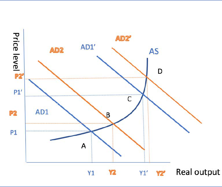
ECB Forum on Central Banking, November 2020
235
Chart 6
Fiscal policy in theory: expansions versus recessions
The AS-AD model and the effects of an increase in government spending in recessions
versus expansions
Notes: Fiscal policy in recessions vs. expansions.
On the theoretical front, Canzoneri et al. (2016) propose a model that features costly
financial intermediation and countercyclical financial frictions which generate state-
dependent effects of fiscal policy similar to those presented above. In their model, a
fiscal expansion during a recession may lead to multiplier values exceeding two,
while a similar expansion during an economic boom would produce multipliers falling
short of unity.
Contrary to the conventional wisdom, only a few dynamic stochastic general
equilibrium models can deliver higher output multipliers from government spending
shocks in recessions. Moreover, the evidence for higher spending multipliers during
recessions is fragile, and the most robust results suggest multipliers of one or below
during these periods (see also Ramey (2019)). This is really discouraging since it
points to the inability of government spending alone to fight recessions. It must be
noted that multipliers, though smaller than one, are still positive, which implies that
government spending can still help lift the economy out of a severe recession. Yet, in
order to do so, the amount of government spending needs to be substantial, as has
happened in the past with the World War II government spending that lifted the US
economy out of the Great recession.
Fortunately, the literature has identified instances in which government expenditure
can still be effective in counteracting recessions and I analyze these cases in the
next subsections.

ECB Forum on Central Banking, November 2020
236
2.1.2 Government spending increases are more effective at the zero-
lower bound.
Several New Keynesian DSGE models show that government spending multipliers
can be higher than one when monetary policy is constrained by the zero-lower
bound (ZLB) on interest rates.
Monetary policy can offset the positive effects from the fiscal stimulus in normal
times by reacting to future expected inflation through a rise in interest rates. When
monetary policy reacts to expected inflation in this way, it partially undoes the effects
of the fiscal expansion. In terms again of the simple textbook analysis in Chart 7,
active monetary policy shifts aggregate demand inwards after the fiscal expansion,
moving the economy from point F to point G, reducing the initial impact of the fiscal
expansion. The temporary effectiveness of fiscal policy when monetary policy is
constrained at the lower bound is the most powerful and widely spread argument for
the active use of discretionary fiscal policy in an economic environment of low-
inflation and low-growth.
Chart 7
Fiscal policy in theory: monetary fiscal policy interactions
The AS-AD model and the effects of government spending increases in different monetary
policy regimes
Notes: Fiscal policy with passive and active monetary policy.
Research by Christiano et al. (2011), Canova and Pappa (2011), Eggertson (2011),
Woodford (2011), Coenen et al. (2011), Blanchard et al. (2017), Farhi and Werning
(2016), and Leeper et al. (2017) shows that multipliers increase at the ZLB and with
ECB Forum on Central Banking, November 2020
237
the duration of the government stimulus. The main mechanism in New Keynesian
DSGE models works as follows: as expansionary fiscal policy increases inflation
expectations in a setup where the nominal interest rate is zero, the real interest rate
actually falls. This affects the intertemporal decision problem of the consumers,
leading to higher private spending. Since the latter induces further inflation there is a
reinforcing effect in the fall of the real interest rate, so that fiscal policy becomes
even more effective.
However, other authors have developed theoretical models that predict lower
multipliers at the ZLB. Mertens and Ravn (2014) describe an environment in which a
loss in confidence can set the economy on a deflationary path that eventually
prevents the monetary authority from adjusting the interest rate and can lead to
potentially very large output drops. Contrary to the previous literature, they find that
demand stimulating policies become less effective in a liquidity trap induced by loss
of confidence than in normal circumstances. The key reason is that demand stimulus
leads agents to believe that things are even worse than they thought. In contrast,
supply side policies, such as cuts in labor income taxes, lead to relative optimism
and become more powerful. Aruoba and Schorfheide (2015) illustrate that there is a
multiplicity of inflation and real activity paths around the lift-off from the ZLB. The
existence of multiple equilibria implies that the same monetary or fiscal policy action
of, say, changing interest rates or increasing government spending, may have very
different effects, depending on the equilibrium. For that reason, it is important to
revise once more the empirical evidence in order to draw sound conclusions on the
effectiveness of fiscal policy at the ZLB.
The empirical estimates seem to agree that spending multipliers are higher at the
ZLB. For example, Miyamoto et al. (2018) report estimates in the range of [1.5, 2.5]
at the ZLB for Japan, while Ramey and Zubairy (2018) report estimates of around
1.5 for historical samples in the US.
The existence of strong complementarity between monetary and fiscal policies at the
ZLB might change the way policy is conducted. However, as discussed in the
previous section, large stocks of debt accumulated by some governments during the
prolonged recession dramatically reduce their room for maneuver. As a result, in the
current situation, assessing the trade-off between the active use of a fiscal
expansion – with the potential to boost economic activity and raise inflation – and the
risk of triggering unsustainable public debt dynamics is of key importance (Blanchard
2019). The active use of fiscal policy for stabilization purposes should always follow
a careful assessment of the impact on public debt sustainability. Yet Battistini and
Callegari (2020) present a closed economy model in which they show that this
assessment changes during periods of binding ZLB. A sequence of deficit-financed
public spending shocks during a prolonged period at the ZLB could improve output,
reduce inflation and, at the same time, lower the risk spread compared to a situation
without fiscal expansion. Their model shows that the driver of this concurrent
improvement in macroeconomic stabilization and debt sustainability through an
unanticipated fiscal expansion is the large long-run fiscal multiplier of public
spending in times of binding ZLB, as highlighted by the recent literature. The timing
of the fiscal expansion is crucial in their model. An excessively delayed series of
ECB Forum on Central Banking, November 2020
238
public spending shocks – starting when the risk-free rate is still low but continuing
well into a period when monetary policy can react to inflationary pressures – would
not benefit from the large fiscal multipliers of the ZLB. In effect, a delayed fiscal
expansion could lead to soaring sovereign spreads and debt levels and, eventually,
long-run output losses. As these dynamics would be further amplified in the presence
of higher initial debt levels, the right timing for a fiscal expansion is crucial, especially
for highly indebted countries.
Hence, our analysis suggests that discretionary fiscal policy can work at the ZLB, yet
one should not undervalue the role of sentiments and the debt level as crucial factors
for determining the success of the fiscal-monetary policy mix.
2.1.3 The multiplier for government spending in monetary unions
In a monetary union, monetary policy is also constrained as it does not directly react
to the actions of regional fiscal policy. When monetary policy is conducted at the
central level, or in fixed exchange rate regimes, fiscal policy can be more effective
since the reaction of monetary policy to the inflation pressures is more limited. Farhi
and Werning (2016) show that self-financed multipliers in a currency union are
always below unity, unless the accompanying tax adjustments involve substantial
static redistribution from low to high marginal propensity to consume agents, or
dynamic redistribution from future to present non-Ricardian agents. Yet, outside-
financed multipliers, which require no domestic tax adjustment, can be large,
especially when the average marginal propensity to consume on domestic goods is
high or when government spending shocks are very persistent. Iltzetzki et al. (2010)
and Born et al. (2013) find higher estimates of multipliers in fixed versus flexible
exchange rate regimes. Nakamura and Steinsson (2014), estimate the effect that an
increase in government spending in one region of the union (relative to another
region) has on relative output and employment. To estimate these effects, they use
variations in historical regional military procurement associated with aggregate
military build-ups. They find that when relative per capita government purchases in a
region rise by 1 percent of regional output, relative per capita output in that region
rises by roughly 1.5 percent. The insight into why the regional relative multiplier is
larger than the closed economy aggregate multiplier in the U.S. is similar to the
intuition explaining why the government spending multiplier is larger under a fixed
than a flexible exchange rate in the Mundell-Fleming model. Economies which
maintain an exchange rate peg or belong to a currency union are characterized by
large fiscal multipliers according to this model. Conversely, the multiplier is zero
under a floating exchange rate regime since the increased activity due to higher
government spending puts upward pressure on interest rates, which triggers capital
inflows and leads to an appreciation of the currency. This, in turn, crowds out net
exports and eventually offsets the effect of increased public spending on the demand
for domestic goods. Under fixed exchange rates, in contrast, monetary policy
accommodates the increased demand for domestic currency to prevent the currency
from appreciating. As a result, private demand rises along with public demand, while
net exports remain unchanged and the multiplier exceeds unity.
ECB Forum on Central Banking, November 2020
239
Chodorow-Reich (2019) surveys the estimates of sub-national multipliers for
government purchases, temporary tax rebates, and transfers, reporting multipliers in
the range of 1.5 to 2. Sub-national multipliers tend to be higher than the aggregate-
level ones. In general, the relationship between sub-national multipliers and
aggregate multipliers depends on many features, including how the spending is
financed, whether there are spill-overs across regions, whether there is a currency
union, and whether the aggregate economy is at the ZLB. Canova (2020)
recommends taking the results of these studies with caution.
For example, two studies that look at the size of the regional multiplier at the euro
area come to opposite conclusions using different estimation techniques and
instruments to extract government spending shocks. Following the estimation
methodology of Nakamura and Steinsson (2014) and using shocks to the supply of
federal transfers (European Commission commitments) of structural fund spending
by sub-national regions as instruments for annual realized expenditure in a panel
from 2000-2013, Coelho (2016) finds a relatively high local multiplier across the EU:
1.7 on impact and around 4.0 after three years at the EU cross-regional level. This
author also shows that multipliers are generally higher in the post-2006 period of
economic recession in Europe. By contrast, Bruckner et al. (2020), studying regional
European data and using a standard panel model to estimate the effect that regional
government spending has on regional gross value added, find that regional
multipliers are smaller than one in general and that they depend positively on the
degree of local fiscal autonomy. When they consider state-dependence, they report
multipliers higher than one in the EU regions in recessions and in periods of labor
market slack. Finally, they also show that there are significant spill-over effects
among regions in the same country and that national cumulative multipliers of
government spending shocks are higher than one in European countries.
Canova and Pappa (2007) provide evidence that regional fiscal policy can stimulate
domestic demand for two big monetary unions, such as the USA and the EMU. In
particular, they show that both expansionary government spending and tax cuts
increase regional output, employment and the price level relative to the union
average. It is worth highlighting their finding that using taxes as the fiscal instrument
seems more adequate in the USA, while using government spending as the fiscal
tool seems more adequate in Europe. Yet, Canova and Pappa (2007) reveal that
fiscal policy, when constrained by balance-budget rules, can have significant adverse
real and price effects. More recent work by Amendola et al. (2019), building a factor-
augmented interacted panel vector-autoregressive model of the euro area (EA) and
estimating it with Bayesian methods, computes government spending multipliers in
the EA. The multiplier is inversely correlated with the level of the shadow monetary
policy rate. In particular, they show that the ZLB constraint is crucial for determining
the size of the spending multiplier especially for the medium run. The average three-
year multiplier is about 1 in normal times and between 1.6 and 2.8 at the ZLB,
depending on the specification. Moreover, according also to their estimates, the EA
data support the view that the multiplier is larger in periods of economic slack.
ECB Forum on Central Banking, November 2020
240
To sum up, the literature suggests that regional multipliers for government can be
higher than aggregate multipliers. Additionally, for the euro area there is evidence
pointing to these effects being larger at the ZLB.
2.1.4 Government spending has positive spill-over effects
National fiscal policies spill over to other countries through trade. A fiscal expansion
in one country increases its imports from other countries. It could also increase
domestic prices and the real effective exchange rate, reinforcing spill-overs, as the
stimulating country loses competitiveness vis-à-vis the other countries. Given the
implications of this trade channel for prices, it is important to consider the monetary
policy response. For instance, interest rates may occasionally fail to react to price
changes stemming from fiscal action if the economy is constrained by the ZLB. Spill-
over estimates of public spending tend to be positive, but generally small. A number
of studies have estimated fiscal spill-overs from an increase in public spending
through the trade channel for a panel of countries. For example, based on annual
data from 1965 to 2004, Beetsma et al. (2006) estimate that a spending-based fiscal
expansion of 1% of GDP in Germany would lead to an average increase in the
output of other EU economies of 0.15% after two years; for an expansion originating
in France, the impact is 0.08%. The estimated magnitude of spill-overs varies, with
the heterogeneity related to the trade links, the state of the economy and the
reaction of monetary policy. These authors report spill-overs from Germany to its
neighboring countries (Austria, Belgium and the Netherlands) to be around 0.4% of
GDP after two years. Auerbach and Gorodnichenko (2013) find spill-overs that are
particularly high in recessions and more modest in expansions. IMF (2017) finds that
spill-overs are up to four times as large when monetary policy is at the effective
lower bound (0.3% after one year), compared with normal times (0.08%).
Recent work by Alloza et al. (2020) provide new estimates of fiscal expenditure spill-
overs in the euro area, as well as simulations, to provide a better understanding of
their driving factors. Although effects are heterogenous, they confirm the existence of
positive fiscal spill-overs within euro area countries. Using the Euro Area and Global
Economy (EAGLE) model, Alloza et al. (2020) also show that spill-overs within the
euro area are larger when interest rates do not increase in response to an increase
in government expenditure. Their results square well with the findings of earlier work
by Blanchard et al. (2015). The latter authors, using a simple and a larger-scale
DSGE version of a New Keynesian model of a currency union, show that outside of a
liquidity trap, the effects of higher core government spending on periphery GDP tend
to be small and even negative. The small response of periphery GDP reflects that
the central bank raises real interest rates, more than offsetting the stimulus arising
from a depreciation of the periphery’s terms of trade. These results concur with
previous research by Wieland (1996) and Kollmann et al. (2014) indicating that fiscal
spill-overs tend to be negative under fixed exchange rates (assuming that the central
bank responds according to a standard policy reaction function). However, they also
show that the spill-overs to periphery GDP are markedly different in a liquidity trap:
periphery GDP tends to rise, reflecting the weaker interest rate response. The size of
the periphery GDP response to a core spending hike increases with the expected

ECB Forum on Central Banking, November 2020
241
duration of the liquidity trap, with the import content of core government spending,
and with the responsiveness of inflation. Higher core spending can provide a strong
source of stimulus to the periphery if monetary policy is expected not to raise interest
rates for a prolonged period of a couple of years or more.
Hence, both empirical and theoretical contributions agree that fiscal spill-overs are
important in the euro area and, in particular, when monetary policy is constrained by
the effective ZLB.
2.1.5 Tax and transfer multipliers
During recessions, the government might offer a tax cut as an economic stimulus
instead of raising public spending. The issue of whether tax cuts are more or less
expansionary than increases in public spending is a critical one, and economists
strongly disagree about the answer. The issue is also political. Right-wing politicians
believe in tax cuts and the left wing believes in spending increases.
Again, the empirical evidence is the only reliable way to assess which tools are more
effective. Tax multipliers are generally negative since an increase in taxes lowers
GDP. Evidence presented in Ramey (2019) from different studies suggests that tax
cuts are more expansionary than spending increases. Estimates of cumulative tax
cuts multipliers vary in the [-5, -1.1] interval.
7
Romer and Romer (2010) and Mertens
and Ravn (2012, 2013), using narrative methods to identify tax shocks, report high
multipliers between –2 and –3. Mountford and Uhlig’s (2009) report the highest
estimates (-5) using sign restrictions, while Barro and Redlick (2011) estimate the
lower tax multipliers (around –1.1). Finally, Caldara and Kamps (2017), using a
unified approach to estimate multipliers, suggest that spending increases generate
higher multipliers relative to tax cuts.
The New Keynesian DSGE model estimates of tax cuts multipliers are typically
below one, as Ramey (2019) reports, generating a conflict between the narrative-
based time series estimates and the New Keynesian estimates. This divergence is
present in the work of Coenen et al. (2012) who use seven different structural
models mostly used by policymaking institutions, to simulate the effects of fiscal
stimulus shocks using seven different fiscal instruments. There is a robust finding
across all those models that government spending increases and targeted transfers
to liquidity-constrained individuals have more sizeable output multipliers than tax
instruments.
The literature regarding the expansionary effects of transfers is pretty thin. Coenen
et al. (2012) report multipliers for general transfers in the range of 0.2 to 0.6 and for
targeted transfers around 2. Romer and Romer (2016) construct a series of
legislated increases in social security benefits in the U.S. from 1951 to 1991 and
study the effect of innovations to their narrative variable on private consumption.
7
For the sake of brevity, I refer the interested reader to Table 2 in Ramey (2019)’s paper for a detailed
report of cumulative tax cut multipliers.
ECB Forum on Central Banking, November 2020
242
They find that permanent benefit increases have a significant impact on consumption
upon impact, while temporary increases in benefits have no significant effect on
aggregate consumption.
Párraga Rodríguez (2016) provides evidence on the aggregate effect of government
income transfers shocks using a panel dataset of 22 EU Member States during
2007-2015. She proposes a new measure of transfers shocks based on a dataset by
public finance experts of the ESCB which records discretionary changes in old age
pensions relative to a ‘neutral policy’ benchmark. The estimated old age pensions
output multiplier ranges between 0 and 1, suggesting a limited effectiveness of fiscal
transfers to stimulate the economy.
Unlike the case of spending multipliers, the literature seems to agree on the
asymmetric effects of tax cuts in recessions versus expansions. Demirel (2016),
using the Romer and Romer (2010) narrative tax shocks, finds that tax multipliers
are larger during times of low unemployment than during times of high
unemployment. Also, Alesina, et al. (2018), using narrative of fiscal plans across
OECD countries, report higher multipliers in expansions. Sims and Wolff (2018)
present empirical evidence and develop a model to back up their estimates that
indicate that a tax rate cut is most stimulative for output in periods in which output is
relatively high.
Finally, Correia et al. (2013) provide strong theoretical support on the use of tax cuts
in a closed economy when monetary policy is constrained by the ZLB. These authors
argue that distortionary taxes can be used to replicate the effects of negative
nominal interest rates and completely circumvent the ZLB problem. They label this
scheme “unconventional fiscal policy”. The suggested policy involves engineering
over time an increasing path for consumption taxes and a decreasing path for labor
taxes, coupled with a temporary investment tax credit or a temporary cut in capital
income taxes. Under such a scenario, numerical calibrations indicate that the
magnitude of the tax changes is implementable.
In sum, tax cuts offer promise as an instrument to fight recessions in the data and
can also be an effective tool to replicate the effects of negative interest rates in the
presence of the ZLB in a closed economy model. Transfers seem to be less effective
in stimulating the economy unless they are targeted to financially constrained
households. Yet the conclusion on the efficacy of taxes as an effective fiscal
instrument lies on specific assumptions of the state of the economy. In the next
subsection I discuss some specific circumstances in which taxes can be an effective
countercyclical tool.
2.1.6 Fiscal policy and macroeconomic uncertainty
Macroeconomic conditions are at times uncertain. The onset of the financial crisis in
2008 brought an end to the ‘Great Moderation’ period, making prospects for global
economic growth appear not just weaker, but also more uncertain. The COVID-19
pandemic is changing – or has already changed – our previous definitions of
ECB Forum on Central Banking, November 2020
243
uncertainty because there is no reference case for the COVID-19 crisis in living
memory. It is, then, only natural to ask:
How does uncertainty affect the effectiveness of fiscal policy?
There exist theoretical contributions that help us answer this question. Theoretical
models linking uncertainty to investment and hiring decisions by firms (Bernanke
(1983), McDonald and Siegel (1986), Bloom et al. (2018)) and to precautionary
savings on the consumer side (Basu and Bundick (2017), Fernandez-Villaverde et al.
(2011)) predict that agents respond more mildly to positive policy stimuli because
they adopt a wait-and-see or precautionary behavior.
In the case of tax increases in periods of low macroeconomic uncertainty, agents
may be willing and able to smooth consumption and maintain investment. In
exchange, they may not be able to do so in a high-uncertainty regime, typically
associated with a tightening of the credit conditions for households and firms (see
Arellano et al. (2019) and Gilchrist et al. (2014)).
On the empirical front Alloza (2017), looking at government spending shocks, reports
that the response of output to a fiscal expansion is positive during times of low
uncertainty, but negative (or not significant) during times of high uncertainty. In order
to rationalize the fact that output may fall after a government spending shock, he
explores an economic mechanism where information is scarce or noisy during times
of high uncertainty. In this context, agents are concerned that the economy may take
a downturn and lower their future income. A government spending shock during
times of heightened uncertainty may then simply confirm these pessimistic views,
leading in turn to a decline in consumption and activity.
Bertolotti and Marcellino (2019) explore whether high uncertainty affects the fiscal
stimuli of tax cuts. They find that tax changes of either sign, implemented when
macroeconomic uncertainty is high, always have a harmful effect on GDP. Their
empirical results indicate that the economy reacts more negatively to a tax increase
when ex-ante macroeconomic uncertainty is high and, on the contrary, that tax cuts
are more effective in stimulating the economy in periods of low uncertainty. Finally,
they stress the importance of monetary and fiscal policy interactions in rendering
fiscal policy effective in a high uncertainty regime.
In sum, both theoretical and empirical studies agree that high macroeconomic
uncertainty reduces the expansionary effects of fiscal stimuli both in the case of tax
and spending changes. They also point to the interactions of monetary and fiscal
policy as a crucial factor for enhancing the stimulative effects of expansionary fiscal
shocks.
2.1.7 Fiscal policy and the debt level
Government debt can have both direct and indirect effects on the transmission of
fiscal policy shocks. Sutherland (1997) links debt levels to policy expectations to
explain that a fiscal deficit may not have traditional Keynesian effects related to
ECB Forum on Central Banking, November 2020
244
consumption increases. This would be the case if the current generation expects that
fiscal adjustments would occur within the same generation. With a linear fiscal
reaction function of government spending to debt, Corsetti et al. (2012) find that
private consumption can rise to a government spending increase when agents
expect a government spending reversal.
Romer and Romer (2010) find that the effect of a U.S. tax shock on output depends
on whether the change in taxes is motivated by the government’s desire to stabilize
the debt or is unrelated to the stance of fiscal policy. Favero and Giavazzi (2007)
show that omitting debt can bias the evaluation of the output effects of fiscal policy.
As for the fiscal state-dependent fiscal policy effects, several empirical papers
document more expansionary effects of government spending in low-debt than in
high-debt states. Kirchner et al. (2010) show that higher government debt-to-GDP
ratios in the euro area negatively affected long-term multipliers over the period 1980-
2008. Ilzetzki et al. (2013) also present evidence that fiscal multipliers are lower in
countries with high debt-to-GDP levels. Nickel and Tudyka (2014) find that, at high
levels of the debt-to-GDP ratio, the overall effect on real GDP of an increase in
government expenditure turns negative, crowding out investment. Finally, Fotiou et
al. (2020) find that the output effect of capital income tax cuts is government debt-
dependent: it is less expansionary when debt is high than when it is low.
Overall, theoretical and empirical models agree that high levels of debt undermine
the expansionary effects of fiscal policy irrespective of whether it is conducted
through spending increases or tax cuts.
2.1.8 Can fiscal expansions create jobs?
With the emergence of the COVID-19 crisis policymakers realized that it was
essential to keep employment contracts alive. One of the policies that was
immediately put in place was direct subsidies to small and medium enterprises and
businesses to help them maintain their employees (furlough programs). It is natural
therefore to ask whether fiscal policy can create jobs.
Empirically there has been a plethora of studies investigating the effects of fiscal
policy on employment. Monacelli et al. (2010) study the effect of government
spending on the functioning of the U.S. labor market. Using a structural VAR, they
find that a rise in spending equal to 1% of GDP raises labor market tightness by
around 20% and employment by 1.6%, lowering the unemployment rate by 0.6
percentage points. Recent cross-state studies further corroborate these findings.
Chodorow-Reich et al. (2012) estimate the employment effects of a relatively
unstudied form of government macroeconomic intervention that took central stage in
the recent American Recovery and Reinvestment Act: fiscal relief to states during a
downturn. They exploit the cross-state variation in transfer receipts that comes from
pre-recession differences in Medicaid spending. Their baseline specifications
suggest that $100,000 of marginal spending increased employment by 3.8 job-years,
3.2 of which are outside the government, health and education sectors. Shoag
(2013) finds that $100,000 in government spending added around 4.8 jobs, of which
ECB Forum on Central Banking, November 2020
245
2.5 can be attributed to a reduction in unemployment, with the additional 2.3
stemming from a rise in labor market participation. Bruckner and Pappa (2012) raise
a word of caution by showing that labor force participation, employment, and the
unemployment rate all increase significantly and at the same time in response to
government expenditure shocks in many OECD countries. However, Ramey (2012)
argues that the increase in employment stemming from government expansions
comes from an increase in government employment, not private employment, and
concludes that, on balance, government spending does not appear to stimulate the
labor market. Finally, in comparing tax cuts with government spending increases,
Adnan et al. (2020) show that tax shocks have larger effects, in terms of magnitude
and significance, on the unemployment rate compared to defense spending shocks.
Theoretically, Bruckner and Pappa (2009) and Monacelli et al. (2010) present New
Keynesian DSGE models that can replicate the previous empirical findings.
Interestingly, Rendhal (2016) presents a framework in which equilibrium
unemployment dynamics can significantly enhance the efficacy of fiscal policy. In this
model (with sticky nominal wages) output is largely determined by demand at the
ZLB. As a result, a temporary rise in government spending increases output and
lowers the unemployment rate. Since movements in unemployment are partly
persistent, a reduction on impact is also expected to last into the future.
In sum, the transmission mechanism of fiscal policy appears to be closely intertwined
with the labor market. A rise in government spending seems able to have positive
effects on job creation and to jointly raise both employment and output.
2.1.9 Can increases in government employment be expansionary?
In the U.S. the “public option” for employment (Henceforth, POE, see Bivens (2018))
has gained popularity. According to this doctrine, by providing a public option for
employment, the government becomes an “employer of last resort” for job seekers
who are otherwise unable to find work in the private sector or through existing public
structures. Generally, POE proposals are envisioned as providing a tranche of public
money to states and localities to provide a steady buffer of jobs to those willing
workers who remain locked out of work even after best practice in job creation policy
has been followed. These jobs could be publicly managed, or they could support
work in the non-profit sector.
A characteristic feature of POE proposals is that the job matters more than the
output. The jobs associated with POE programs must be temporary jobs that
disappear once the economy heats up and the private sector pulls people into
employment from the public sector. In this section I review the literature that
analyses the stimulating role of increases in public employment for both output and
employment.
Few papers have analyzed the role of government employment to create jobs and
stimulate the economy. Linnemann (2009) has shown, using aggregate U.S. time
series, that increases in public employment generate positive responses of private
employment and real output and a short-lived expansion in private consumption.
ECB Forum on Central Banking, November 2020
246
Pappa (2009) reports mixed results for the employment response to government
employment shocks using annual U.S. state and aggregate data over the period
1969–2001. Bermperoglou et al. (2017) estimate the macroeconomic effects of
public wage expenditures in U.S. data by identifying shocks to public employment
and public wages using sign restrictions. Their main finding is that public
employment shocks are mildly expansionary at the federal level and strongly
expansionary at the state and local level by crowding in private consumption and
increasing labor force participation and private sector employment. Their model also
predicts that increases in public employment might induce wage inflation in normal
times. This last observation is also reflected in the work of Moscarini and Postel
Vinay (2019) that highlights that when the labor market is tight, expansionary policies
might lead to wage inflation.
Theoretically, Michaillat (2014) develops a New Keynesian model in which the effect
of government policy varies across stages of the business cycle. This author
considers a policy in which the government increases the size of the public-sector
workforce and measures the effect of this policy with the public-employment
multiplier, defined as the additional number of workers employed when one more
worker is hired in the public sector. The main finding is that this multiplier doubles
when the unemployment rate rises from 5 percent to 8 percent. The government
policy reduces unemployment more effectively in a recession than in an expansion
because crowding out is weaker during a recession. The extent of crowding-out is
determined by the amplitude of the increase in labor market tightness. When
unemployment is high, the government needs few vacancies to hire additional
workers because the matching process is congested by job seekers; moreover, the
number of job seekers is so large that the vacancies posted and job seekers hired by
the government have little influence on tightness. Consequently, the increase in
tightness is small and crowding-out is weak. The same mechanism leads to strong
crowding-out when unemployment is low and the matching process is congested by
vacancies.
Overall, increases in public employment can decrease unemployment in the short-
run and especially during recessions. However, in normal times, or when labor
markets are tight they might induce wage inflation as they shift the labor supply from
the private to the public sector, putting pressure on the marginal costs of private
firms.
2.1.10 The promise of government investment
In the last decade, and especially after the sovereign debt crisis, most of the Member
States of the euro area have suffered a considerable reduction in public investment.
Chart 8 displays the evolution of government investment-to-GDP ratio between
2006Q1 and 2019Q3 in Germany, France and the Netherlands and in Spain, Italy,
Greece and Portugal.
The cuts in public investment in the European periphery were devastating. Starting
from an average of 4.1 percent of GDP between 2000 and 2007, public investment

ECB Forum on Central Banking, November 2020
247
fell to 2.38 percent of GDP afterwards in the periphery countries. On the contrary, the
cuts in government spending in investment have been less pronounced in France
and the Netherlands, whereas public investment in Germany was never affected by
the sovereign debt crisis. In this section, I review the available literature on the
macroeconomic role of government investment in order to evaluate whether those
cuts were detrimental and the extent to which government investment can be used
as a useful tool for fiscal stimuli. I also provide new insights about the effects of
government investment shocks.
Chart 8
Government investment as a percentage of GDP 2006-2019
Evolution of government investment as a share of GDP 2006-2019, selected EA countries
(share of government gross fixed capital formation to GDP, years)
Sources: Eurostat.
Pappa (2009) is one of the first papers that looks at the effects of shocks to
government investment on the macroeconomy. Using data from the U.S. and sign
restrictions in a SVAR model for shock identification, it is found that shocks to
government investment increase output and the real wage persistently, and they
have a positive, significant, but short-lived effect on private employment. Those
findings are rationalized through the lenses of a DSGE model with price stickiness in
which government investment increases the stock of public capital which, in turn,
enhances private production. Basically, a government investment shock, apart from
stimulating demand through the standard Keynesian channel, has an additional
supply side effect that works through the production function when, as in the seminal
work of Aschauer (1982 and 1989), public capital is assumed to be productive. In
terms of the basic textbook analysis presented earlier, an increase in government
investment implies a shift of both the aggregate demand and the aggregate supply to
the right, from point H in Chart 9 to point K. However, since capital needs time to
build, the movement from point J to point K takes time and this is why increases in
government investment tend to generate persistent output increases.
0
1
2
3
4
5
6
Q1-2006
Q3-2006
Q1-2007
Q3-2007
Q1-2008
Q3-2008
Q1-2009
Q3-2009
Q1-2010
Q3-2010
Q1-2011
Q3-2011
Q1-2012
Q3-2012
Q1-2013
Q3-2013
Q1-2014
Q3-2014
Q1-2015
Q3-2015
Q1-2016
Q3-2016
Q1-2017
Q3-2017
Q1-2018
Q3-2018
Q1-2019
DE
FR
NL
AU
IT
GR
PT
ES

ECB Forum on Central Banking, November 2020
248
Chart 9
Fiscal policy in theory: an increase in government investment
The AS-AD model and the effects of an increase in government spending in investment
Notes: Increases in government investment.
In a recent paper, Ramey (2020) revives the interest in research for analyzing the
effects of government spending on infrastructure by reviewing the existing literature
and putting out a call for new research on the subject. The existing results support
the positive long-run effects of infrastructure investment. Ramey (2020) provides
theoretical analysis and empirical estimates that cast doubt on the positive short-run
effects of infrastructure investment. In particular, she considers more realistic
features of infrastructure investment, such as time to build and sector-specific
demand effects, showing that those additional assumptions actually reduce the
short-run aggregate stimulus effects of shocks to infrastructure investment, even
when the long-run supply-side benefits are present. Earlier work by Leeper et al.
(2010) shows that implementation delays can make the economic benefits from
government investment difficult to synchronize with the business cycle. More
specifically, as long as public capital is productive, the expectation of higher
infrastructure spending generates a positive wealth effect, which discourages work
and encourages consumption. Because private investment projects typically do not
entail the substantial delays associated with public projects, it takes less time to build
private capital. Private investment and employment, therefore, may be delayed until
the public capital is built and raises the productivity of private inputs. Hence, in their
model, increases in public infrastructure result in negative employment and private
investment responses. Boehm (2020) also warns against using investment in public
infrastructure as a short-run stabilization tool. His estimates on the fiscal multiplier
ECB Forum on Central Banking, November 2020
249
associated with government investment during the Great Recession are close to
zero, while the corresponding estimate for government consumption multiplier is
around 0.8. The investment multiplier is small because private investment falls
drastically after government investment shocks. This high degree of crowding out is
driven by the high intertemporal elasticity of substitution of investment demand,
which has been shown to be a feature of a large class of macroeconomic models
(see, e.g., Mankiw (1985)). Ramey (2020) also highlights the importance of the initial
level of public capital relative to the socially optimal level. Long-run multipliers are
higher if the economy is starting below the optimal level of public capital.
When I turn to the empirical evidence, the short-run effects of investment in public
infrastructure are still debatable. Pappa (2009) estimates positive short and long run
effects from public spending and Bruckner and Pappa (2015) provide additional
evidence that news about infrastructure investment associated with the hosting of
the Olympic games actually significantly increases private investment, consumption,
and output. On the other hand, Boehm (2020) calculates the government investment
multiplier to be practically zero. Thus, further empirical work is needed to evaluate
the short-run effects of investment in infrastructure on the macroeconomy.
In total, although there is no doubt about the growth-enhancing effects of
government investment increases, its use as a short-term stabilization tool is the
subject of a current academic debate and possible future empirical work.
3 The Recovery Fund and it’s possible effectiveness
July 21, 2020 will be considered a historical date for the European Union (EU). On
that date, the European Council has agreed to a new EU budget for 2021-2027
which, for the first time ever, includes funds that do not only come from national
contributions but are also borrowed from international financial markets. The Council
has made provisions to back the current borrowing with taxes on future carbon
emission, plastic use and financial transactions, among others. Thus, an embryo of
federal fiscal policy has been created. Apart from the regular budget (named Multi
Annual Financial Framework), the agreement allows for the Next Generation EU
(NGEU) funds, a new package of programs which, through a combinations of grants
and loans to member states attempts to support the recovery from the COVID-19
pandemic and foster investment, leading to the transformation to a green digital
economy.
The largest instrument among the NGEU funds, the Recovery and Resilience Facility
(RRF), has been especially designed to counteract the negative economic effects of
COVID-19 and help countries in difficulties by providing part of the funds national
governments borrowed to help workers and firms. It should also facilitate the
recovery, hopefully back to the growth path existing prior to the pandemic, by
creating jobs and incentivizing the transformation of the EU economy to sectors and
activities with large strategic potential. The expected fiscal expansion is huge. The
total budget for the RRF is 750 billion euros which amounts roughly to 5.7 percent of
gross national income (GNI) of the EU. Will this effort succeed in creating jobs? Will

ECB Forum on Central Banking, November 2020
250
the EU economy recover fast from the pandemic shock? Will the conversion to a
greener economy be smooth? Will the programs start a virtuous growth cycle?
Questions of this type loom in the back of the mind of policymakers and academic
economists. While expectations are optimistic, the large costs and the uncertain
benefits of the proposed programs, and the unequalled nature of the current
economic situation, call for caution and care in thinking about the economic
consequences of the fiscal expansions the EU is planning to undertake.
The existing literature supports the idea that large fiscal expansions can work to
smooth the cycle. The analysis in the previous sections has revealed that fiscal
policy expansions at the ZLB have the potential to push the economy out of a
recessionary path with relatively little effort. However, macroeconomic uncertainty
and low sentiment might counteract the effects of the fiscal expansion. I have also
argued earlier that some policies could work better than others. For example, there is
little controversy about the long-run effects of increases in public investment.
However, the literature points to a weak role of government investment to smooth
cyclical fluctuations. Letting the government act as an employer of last resort and
creating jobs when labor market conditions are slack, might also help the economic
recovery.
It is worth highlighting that the kind of fiscal expansion considered with the Next
Generation EU (NGEU) fund is not unprecedented in the euro area. EU policy has
been targeting, for 30 years now, all regions of the European Union with the goal of
supporting job creation, business competitiveness, economic growth, sustainable
development, and improving the quality of life of EU citizens. To reach these goals
and to deal with the heterogeneous stages of development of different EU regions, a
portion of the total EU budget is set aside for the so-called Cohesion policy in each
budget cycle. For example, for the 2014-2020 cycle the Cohesion policy program
was endowed with over 355 billion Euros, almost a third of the total EU budget.
The European Structural and Investment funds, which are the main tools to achieve
the Cohesion policy goals, include four different programs: the European Regional
Development Fund (ERDF), the Cohesion Fund (CF), the European Social Fund
(ESF), and the European Agricultural Fund for Rural Development (EAFRD)
8
. The
ERDF fund covers over 40 percent of the total budget, the EAFRD fund over 20
percent, and the ESF and CF funds less than 20 percent each.
Canova and Pappa (2020) provide evidence of the dynamic macroeconomic effects
of structural funds that the EU granted to member states (and regions) over the last
30 years. Thus, they offer some historical perspective to evaluate the likelihood of
the success of the planned fiscal expansion. To gather information about the likely
consequences of the planned fiscal expansion, they focus on the production,
employment, productivity, investment, and real wage effects of the grants provided
by two funds: (i) the Regional development fund (ERDF), whose aim is to foster
investments in innovation and research, to favor the digital agenda and to support
8
In the most recent budget cycle, the European Maritime and Fisheries Fund (EMFF) has been added.

ECB Forum on Central Banking, November 2020
251
small and medium-sized enterprises; and (ii) the European Social Fund (ESF),
whose aim is to support investments in education and health, and to fight poverty.
To examine the dynamic effect of ERDF and ESF grants on regional macroeconomic
variables Canova and Pappa (2020) employ local projections. Given the potential
endogeneity of structural funds to EU economic conditions, they use as an
instrument in the projection equations their innovations, constructed as the residuals
of a regression of each real structural fund series on a constant and four aggregate
euro area variables: GDP, employment, GDP deflator, nominal interest rate, and
nominal effective exchange
rate. The dependent variable in local projection is the
cumulative growth rate at horizon h of each macroeconomic variable of interest,
i.e, y
,,
=
,
,
,
. The independent variable is the cumulative change in
the relevant grant, scaled by regional GVA
9
, i.e., x
,,
=
,
,
,
. This way,
and consistent with the literature, see e.g. Ramey and Zubairy (2018), the
coefficients on x
,,
can be interpreted as the cumulative multipliers of the fund
grants (Euro change in private income per Euro of grants) at each horizon h. As
controls in the projection equation, they use a constant and one lag of the dependent
variable. Formally, for each macroeconomic variable, the local projection is:
y
,,
= a
,
+ b
,
y
,,
+ c
,
x
,,
+ e
,,
(3)
where i refers to region, t to time, h to the horizon. The instrumental variable
regression is:
x
,,
=
,
+
,
w
,
+ u
,,
(4)
where w
,
are aggregate euro area variables defined above. They use u
,,
as
instrument for x
,,
in (3). Thus, c
,
represents the cumulative multiplier at horizon h
of an unexpected increase in a structural fund. Given the short size of the available
annual time series, they limit attention to h=1,2,3 and do not use among the controls
lags of other regional variables.
There are two important conclusions that Canova and Pappa (2020) reach. First,
they show that the grants accrued to the regions through the two funds have very
different effects. Table 2 reports the one, two and three-year cumulative average
multipliers for the six regional macroeconomic variables of interest, separately for
ERDF and ESF grants.
The ERDF funds have an important positive short-term (one year) effect on all
regional macroeconomic variables, making them potentially useful for rapid
countercyclical policies. However, the positive regional impact dies out quickly and
private sector gains dissipate within three years. On the other hand, the ESF funds
take a while to exercise their effect, making them good candidates to achieve
medium term objectives. The ESF grants have a positive medium-term impact on
investment, production and workers’ compensation, but smaller effects on
employment.
9
They choose to scale the grant variable by regional GVA rather than regional income since the
measurement of the regional component of the public sector is problematic in this dataset.

ECB Forum on Central Banking, November 2020
252
Table 2
Average cumulative multipliers from European structural and investment funds
Average cumulative multipliers for ERDF and ESF funds
(macro variables, multipliers at different horizons)
Macroeconomic variables, ERDF funds ESF funds
1 year 2 years 3 years 1 year 2 years 3 years
GVA
2.42
(0.19)
1.56
(0.32)
0.56
(0.32)
-0.14
(0.63)
2.70
(0.79)
5.05
(0.82)
Employment
0.86
(0.15)
-0.03
(0.27)
-0.42
(0.29)
-0.33
(0.23)
-0.62
(0.34)
0.96
(0.36)
Investment
8.07
(1.71)
0.53
(2.68)
-1.40
(2.69)
2.13
(1.65)
2.75
(1.63)
3.58
(1.88)
Labor productivity
3.66
(0.37)
-3.65
(0.78)
-4.45
(0.75)
4.09
(0.70)
0.22
(0.83)
3.26
(0.85)
Real Compensation
3.85
(0.36)
-2.62
(0.85)
-4.50
(0.84)
2.95
(0.32)
-1.54
(0.62)
4.54
(0.69)
Sources: Canova and Pappa (2020)
Notes: Standard errors are in parenthesis
The average numbers reported in Table 2 mask considerable regional heterogeneity
of outcomes. For example, at the three years horizon, the interquartile range of
individual GVA multipliers generated by ERDF grants is [-5,5] and the interquartile
range of employment multipliers is [-1.5, 0.3].
To examine whether the regional heterogeneity in multipliers is linked to interesting
characteristics, Canova and Pappa (2020) cluster estimates using a number of
indicators. First, they cluster them using national borders. If, say, labor market
institutions matter, then regions belonging to a country should exhibit a more
homogeneous response to the grants’ stimulus and should display sign and
magnitude similarities in terms of GVA and employment multipliers. Charts 10 and 11
map the joint distribution of GVA and employment multipliers at the three-year
horizon for the two different funds.
The second conclusion is that funds have not affected European countries in the
same way. When looking at ERDF funds for Spain, France, Italy, Ireland, the
Netherlands, Finland, Latvia and Romania the average cumulative multiplier is
positive and significant both for GVA and employment, while for the UK, Belgium,
Estonia, Greece, Cyprus, Bulgaria, Austria, Germany, Poland, the Czech Republic,
Slovakia and Slovenia they estimate negative multipliers for both employment and
GVA.
Particularly interesting for the NGEU effectiveness is the fact in three of four major
Euro countries (Spain, Italy and France) ERDF and ESF grants do create jobs and
increase private sector GVA leading to productivity improvements. In the UK, the
country with the largest number of regions, three-year cumulative employment and
GVA multipliers are instead negative for both types of funds.

ECB Forum on Central Banking, November 2020
253
Chart 10
3-year cumulative ERDF GVA and employment multipliers across national borders
Source: Canova and Pappa (2020).
Chart 11
3-year cumulative ESF GVA and employment multipliers across national borders
Source: Canova and Pappa (2020).
ECB Forum on Central Banking, November 2020
254
Finally, multipliers for Germany, the country with the second largest number of
regions, closely follow the patterns of Table 2: three-year cumulative employment
multipliers are generally negative; three-year cumulative GVA multipliers are
negative for ERDF grants and positive for ESF grants. Similar to ESF grants, when a
country displays a positive and significant cumulative three-year employment
multiplier, it also displays a large and positive three years cumulative GVA multiplier
(Spain, Italy, France, Denmark, Hungary, Finland).
These differences cannot be explained by standard political and economic structural
differences, such as differences in institutions, labor market structure, or degrees of
corruption and quality of governance. Identifying possible factors that explain the
remarkable performance of the regional funds in France, Italy and Spain and Finland
and Romania is the subject of our current research. Yet it is important to note that the
latter three countries are those which suffered most from the COVID-19 pandemic.
Thus, it is reassuring to observe positive multipliers in those countries for programs
which have similarities to those launched by the European Council in July 2020.
In sum, ERDF grants have an important countercyclical role in the regional
economies, but their macroeconomic effects are quite temporary and the medium
term investments and job creation effects of the grants on the average region are
quite limited. On the other hand, ESF grants do not have strong countercyclical
properties, but have economically significant medium-term effects on the average
growth rate of private output, investments and productivity, a statistically significant
influence on the growth rate of employment, and contribute to increase workers’
compensation. It should be stressed that there are significant differences in the
dynamics these grants induce depending on the economic, geographical and
institutional characteristics of the regions. Hence, the transformation of the EU
economy will be not be uniform and some regions risk being left behind.
4 Conclusions
We started the analysis by revising the European fiscal framework and its
development in the recent years. Fiscal rules are complex and ever evolving in the
European Monetary Union. Their strictness and occasional violations have increased
political uncertainty in Europe. When assessing their efficiency in reducing the debt
burden, we have found fiscal rules related to expenditure expenses to be the most
effective in reducing the accumulation of debt. Such rules decrease the growth rate
of debt-to-GDP by 6.4 percent, while balanced-budget and deficit rules decrease the
accumulation of debt by around 2 percent each. Those results square well with the
proposal of the EFB (2020) for the reform of the Fiscal Framework of using an
expenditure rule to achieve a debt target.
Next, we have characterized optimal fiscal rules and highlighted that countries with
high but moderate levels of debt, such as Finland, the Netherlands and Germany,
seem to comply with the optimal fiscal rule of constant average debt-to-GDP. On the
one hand, debt growth increased in both the 2001 and 2008 recessions and
decreased during the expansions in these countries. On the other hand, countries
ECB Forum on Central Banking, November 2020
255
with large accumulated debts as a share of GDP, such as Italy, Greece Spain and
Portugal, do not seem to behave optimally, possibly because of the presence of strict
fiscal rules and the urge to consolidate after the sovereign debt crisis.
We continue the analysis by highlighting the benefits of discretionary fiscal policy,
especially in times when monetary policy is constrained by the effective lower bound
in interest rates. The review of the existing literature reveales the strengthens and
weaknesses of fiscal policy as a stabilization tool and identifies those fiscal policy
tools that can be more effective as countercyclical buffers relative to other tools that
can have more long-lasting effects.
Finally, we have focused attention on the effectiveness of the fiscal expansion
designed by the Next Generation EU. We bring good news for both economists and
policymakers, as we show that such funds can work. Funds whose aim is to foster
investments in innovation and research, to favor the digital agenda, and to support
small and medium-sized enterprises have an important positive short-term (one
year) effect on all regional macroeconomic variables, making them potentially useful
for rapid countercyclical policies. Funds whose aim is to support investments in
education and health, and to fight poverty, are effective only in the medium run.
However, the presented historical evidence suggests that the new funds will not have
uniform regional effects, nor help those who currently lag the most behind to catch
up.
Finally, we cannot talk about fiscal stimulus and fiscal and monetary policy
interactions without reference to the debt dynamics. One way or another, any
strategic change must calibrate monetary and fiscal policy to an environment of high
debt. Achieving and maintaining an accommodative fiscal policy stance has proved
difficult in the euro area. The decision of the European Council on July 21, 2020 has
opened new avenues for the evolution of fiscal policy in Europe. It does so by
including funds that do not only come from national contributions but are also
borrowed from international financial markets, creating an embryonic federal fiscal
policy. Still, debt issued by national fiscal authorities in the euro area is subject to the
risk of default or restructuring and for some countries in Europe the level of national
debt is dangerously high. The Achilles heel of Europe’s financial markets remains the
high level and risky nature of (national) government debt.
Fiscal accommodation can give rise to expectations of default or restructuring that
counteract or reverse any initial stimulative effects. To make matters worse, the
expectations of default or restructuring can be self-fulfilling. The ECB responded
promptly to the COVID-19 crisis: on March 18, the ECB launched the €750
billion Pandemic Emergency Purchase Program (PEPP), which will last until the
coronavirus crisis period is over but, in any case, at least until the end of 2020. The
assets to be bought under the PEPP are mostly the same: the biggest amount goes
to national and regional government bonds, supra-national debt, and various types of
private sector bonds. On June 4, the ECB increased the maximum size of its
purchases of government bonds under PEPP by €600 billion to €1350 billion and
extended the horizon for those purchases at least to the end of June 2021. The ECB
also emphasized that it wants to maintain flexibility in the purchases across asset
classes and among jurisdictions. Through the PEPP, the ECB aimed, in part, to
ECB Forum on Central Banking, November 2020
256
reduce widening spreads in government bonds for countries like Italy and Spain.
Although the launching of the PEPP has reduced the possibility of self-fulfilling
creditor runs on a euro area member state, the program is designed to safeguard
appropriate monetary policy transmission and not to facilitate fiscal accommodation.
Corsetti et al. (2016) describe a benchmark institutional setup that would make it
possible for the euro area to implement effective stabilization policy. This institutional
setup has two key features. The first one is the introduction of a non-defaultable
Eurobond issued by a “euro area fund,” similar to the European Stability Mechanism.
Along the same lines, according to the theoretical model of Jarocinski and
Mackowiak (2017), the euro area is a “land of indeterminacy”, where macroeconomic
outcomes can be turned around by a single speech, or by announcing policies that
are never implemented. These authors suggest the use of a non-defaultable public
debt instrument as a macroeconomic stabilization device requiring only a fairly
modest degree of centralization of fiscal decision-making among the euro area
member states. The second feature is the ability of euro area member states to be
able to restructure national public debt as a last resort in an orderly way. They have
to do so, without prejudice to full participation in the European Union or the euro, and
with the fund being treated equally with private creditors in case a member state
failed to meet the fiscal criteria and was unable or unwilling to borrow exclusively
from private creditors. The fund would stand ready to resume lending after national
public debt had been restructured, as soon as the member state satisfied the fiscal
criteria again. The COVID-19 crisis has already put the first element of this
institutional setup on the table. The EFB (2020) also proposes the creation of a
permanent fiscal authority. European leaders and policy makers should also consider
bringing in the second element along the difficult road to recovery from the pandemic
crisis.
References
Adams, K. and Bill, R. (2014), “Distortionary fiscal policy and monetary policy goals,”
Economics Letters, Vol. 122, No.1, pp. 1-6.
Adnan, W. Arin, P., Corakci, A. and Spagnolo, N. (2020), “Does fiscal policy favor
some over others?” mimeo.
Alesina, A. and Ardagna, S. (2010), “Large changes in fiscal policy: taxes versus
spending,” in Tax Policy and the Economy, Vol.24, pp. 35-68, NBER, Jeffrey R.
Brown.
Alesina, A. and Passalacqua, A. (2016), “The political economy of government debt”.
Handbook of Macroeconomics, Vol. 2, pp. 2599-2651, North Holland.
Alesina, A., Azzalini, G. Favero, C. Giavazzi, F. and Miano, A. (2018), “Is it the ‘how’
or the ‘when’ that matters in fiscal adjustments?” IMF Economic Review, Vol.66, No1,
pp. 144-88.
ECB Forum on Central Banking, November 2020
257
Alloza, M. (2017), “Is fiscal policy more effective in uncertain times or during
recessions?” Banco de España Working Paper, 1730.
Alloza, M., Ferdinandusse, Jacquinot, P. and Schmidt, K. (2020), “Fiscal expenditure
spill-overs in the euro area: an empirical and model-based assessment”, ECB
Occasional Paper, No. 240.
Amendola, A. di Serio, M. Fragetta, M. and Melina, G. (2019), “The Euro-Area
government spending multiplier at the effective lower bound,” IMF Working Paper,
No. 19/133.
Arellano, C., Bai, Y. and Kehoe, P. (2019), “Financial frictions and fluctuations in
volatility,” Journal of Political Economy, Vol 125, No.5.
Aruoba,B. and Schorfheide, F. (2015), “Inflation during and after the zero lower
bound,” Jackson Hole Symposium Volume, Federal Reserve Bank of Kansas City,
2016, 359-436.
Aschauer, D. A. (1989), “Is public expenditure productive?” Journal of Monetary
Economics, Vol. 23, No.2, pp. 177–200.
Auerbach, A. J. and Gorodnichenko, Y. (2012), “Measuring the output responses to
fiscal policy.” American Economic Journal: Economic Policy, Vol. 4, No. 2, pp. 1–27.
Barnichon, R., Debortoli, D. and Matthes, C. (2020), “Understanding the size of the
government spending multiplier: It’s in the sign,” Barcelona GSE Working
Paper, 1145.
Barro, R. J., and Redlick, C.J. (2011), “Macroeconomic effects from government
purchases and taxes.” Quarterly Journal of Economics, Vol.126, No. 1, pp. 51–102.
Basu S., and Bundick, B. (2017), “Uncertainty Shocks in a Model of Effective
Demand”, Econometrica, Vol.85, No. 3, pp.937-958.
Battistini, N. and Callegari, Z. (2020), “Public spending at the effective lower bound:
how significant are the sustainability risks?”, ECB Research Bulletin, No. 67.
Beetsma, R. and Bovenberg, A.L. (1998) “Monetary union without fiscal coordination
may discipline policymakers,” Journal of International Economics, Vol.45, pp. 239–
258.
Beetsma, R., and Uhlig, H., (1999) “An analysis of the Stability and Growth Pact,”
Economic Journal, Vol. 109, No.458, pp. 546–571.
Beetsma R., Giuliodori M. and Klaassen F. (2006), "Trade spill-overs of fiscal policy
in the European Union: a panel analysis", Economic Policy, Vol. 21, No .48, pp. 639-
687.
Beetsma, R., Thygesen, N., Cugnasca, A., Orseau, E., Eliofotou, P. and Santacroce
S. (2018), “Reforming the EU fiscal framework: A proposal by the European Fiscal
Board”, VoxEU.org, 26 October.
ECB Forum on Central Banking, November 2020
258
Bénassy-Quéré, A., Brunnermeier, M., Enderlein, M., Farhi, E., Fratzscher, M.,
Fuest, C., Gourinchas, P.O., Martin, P., Pisany-Ferry, M., Rey, H., Schnabel, I.,
Veron, N., Weder di Mauro, B. and Zettelmeyer, J. (2018), “Reconciling risk sharing
with market discipline: A constructive approach to euro area reform,” CEPR Policy
Insight, No.91, January 2018.
Bermperoglou, D., Pappa, E. and Vella, E. (2017), “The Government Wage Bill and
Private Activity”, Journal of Economic Dynamics and Control, Vol. 79, pp. 21-47.
Bernanke, B. (1983), “Irreversibility, uncertainty, and cyclical Investment,” Quarterly
Journal of Economics, Vol. 98, No.1, pp.85-106.
Bertolotti, F. and Marcellino, M. (2019), “Tax shocks with high and low uncertainty,”
Journal of Applied Econometrics, Vol.34, No.6, pp. 972-993.
Bivens, J. (2018), “Recommendations for creating jobs and economic security in the
U.S.,” Economic Policy Institute Report, No.142207.
Blanchard, O. J. (2019), “Public debt and low interest rates”, American Economic
Review, Vol. 109, No.4, pp. 1197-1229.
Blanchard, O. (1990), “Suggestions for a new set of fiscal indicators”, OECD
Economics Department Working Paper, No. 79.
Blanchard, O. J., Erceg, C. J., and Linde, J. (2017), “Jump starting the euro area
recovery: would a rise in core fiscal spending help the periphery”, NBER
Macroeconomic Annual, University of Chicago Press, Vol. 31, No.1, pp 103-182.
Blanchard, O.J., Á. Leandro, S. Merler and Zettelmeyer, J. (2018), “Impact of Italy’s
draft budget on growth and fiscal solvency”, Peterson Institute for International
Economics, Policy Brief 18-24.
Bloom N., Floetotto, M., Jaimovich, M., Saporta-Eksten, I. and Terry, S. (2018),
“Really uncertain business cycles,” Econometrica, Vol.86, No.3, pp. 1031–1065.
Brückner, M. and Pappa, E. (2012), "Fiscal expansions, unemployment, and labor
force participation”, International Economic Review, Vol. 53, No. 4, pp. 1205–1228.
Brückner, M. and Pappa, E. (2015), “News shocks in the data: Olympic Games and
their macroeconomic effects”, Journal of Money, Credit and Banking, Vol. 47, No. 7,
pp. 1339-1367.
Boehm, C. E. (2020), “Government consumption and investment: Does the
composition of purchases affect the multiplier?” Journal of Monetary Economics,
forthcoming.
Bohn, H. and Inman, R., (1996),” Balance budget rules and public deficits: evidence
from the US”, Carnegie Rochester Conference Series in Public Policy, Vol.45, pp.13-
76.
ECB Forum on Central Banking, November 2020
259
Born, B., Juben, F. and Muller, G. (2013), “Exchange rate regimes and fiscal
multipliers,” Journal of Economic Dynamics and Control, Vol. 37, No. 2, pp. 446-465.
Buti, M., Pench, L., Weale, M., Enderlein, H., Begg, I. and Schelkle, W. (2004),
“Reforming fiscal policy co-ordination under EMU: What should become of the
stability and growth pact?” Journal of Common Market Studies, Vol. 42, No. 5, pp.
1023-1024.
Caldara, D. and Kempfs, C. (2017), “The analytics of SVARs: A unified framework to
measure fiscal multipliers,” Review of Economic Studies, Vol. 84, No. 3, pp. 1015–
1040
Canova, F. (2020), “Should we trust cross sectional multiplier estimates?”, mimeo, BI
Norwegian Business School.
Canova, F. and Pappa, E. (2004), “Does it cost to be virtuous? The macroeconomic
effects of fiscal constraints”, NBER International Seminar on Macroeconomics 2004,
The MIT Press, (edited by R. Clarida, J.Frenkel, F. Giavazzi and K. West).
Canova, F. and Pappa, E. (2006), "The elusive costs and the immaterial gains of
fiscal constraints", Journal of Public Economics, Vol. 90, No. 8-9 , pp. 1391-1414.
Canova, F. and Pappa, E. (2007), “Price Dispersions in Monetary Unions: The Role
of Fiscal Shocks”, Economic Journal, Vol. 520, No. 117, pp. 713-737.
Canova, F. and Pappa, E. (2011), “Fiscal policy, pricing frictions and monetary
accommodation,” Economic Policy, Vol. 26, No. 68, pp. 555-598.
Canova, F. and Pappa, E. (2020), “What are the likely macroeconomic effects of the
EU Recovery plan?”, mimeo.
Canzoneri, M., Cumby, R. and Diba, B. (2002), “Should the European Central Bank
and the Federal reserve be concerned about fiscal policy?” Proceedings - Economic
Policy Symposium - Jackson Hole, Federal Reserve Bank of Kansas City, pp. 333-
389.
Canzoneri, M., Collard, F., Dellas, H. and Diba, B. (2016), “Fiscal multipliers in
recessions.” Economic Journal, Vol.126, No. 590, pp. 75–108.
Carlstrom, C.T., Fuerst, T. S. and Matthias, P. (2014), “Fiscal multipliers under an
interest rate peg of deterministic versus stochastic duration”. Journal of Money Credit
Banking. Vol. 46, No. 6, pp. 1293-1312.
Chari, V.V. and Kehoe, P. (2007), “On the need for fiscal constraints in a monetary
union,” Journal of Monetary Economics, Vol.54, No.8, pp. 2399-2408.
Chodorow-Reich, G. (2019), “Geographic cross-sectional fiscal spending multipliers:
what have we learned?” American Economic Journal: Economic Policy, Vol.11, no. 2,
pp. 1-34.
ECB Forum on Central Banking, November 2020
260
Chodorow-Reich, G., Feiveson, L., Liscow, Z. and Woolston, W.G. (2012), “Does
state fiscal relief during recessions increase employment? Evidence from the
American Recovery and Reinvestment Act.” American Economic Journal: Economic
Policy, Vol.4, No.3, pp. 118-45.
Christiano, L., Eichenbaum, M. and Rebelo, S. (2011), “When is the government
spending multiplier large?” Journal of Political Economy Vol. 119, No 1, pp. 78-121.
Coelho, M. (2019), “Fiscal stimulus in a monetary union: evidence from eurozone
regions”, IMF Economic Review, Vol. 67, pp. 573-617.
Coenen, G., Erceg,C.J., Freedman,C., Furceri, D., Kumhof, M., Lalonde, R. Laxton,
D., Lindé, J., Mourougane, A. Muir,D., Mursula, S., Resende, C., Roberts, J., Roeger,
W., Snudden, S., Trabandt, M. and Veld, J. (2012), “Effects of Fiscal Stimulus in
Structural Models”, American Economic Journal: Macroeconomics, Vol. 4, No.1, pp.
22–68.
Correia, I., Farhi, E., Nicolini,J.P. and Teles, P. (2013), “Unconventional Fiscal Policy
at the Zero Bound”, American Economic Review, Vol.103, No.4, pp. 1172-1211.
Corsetti, G., Meier, A. and Muller, G. J. (2012), “Fiscal stimulus with spending
reversals,” Review of Economics and Statistics, Vol. 94, No.4, pp. 878–895.
Corsetti, G., Dedola, L., Jarocinski, M., Maćkowiak, B. and Schmidt, S. (2016),
“Macroeconomic Stabilization, Monetary-Fiscal Interactions, and Europe's Monetary
Union,” ECB Working Paper, No. 1988.
Debrun, X., Eyraud, L., Hodge,A., Lledo,V. and Pattillo, C. (2018), “Second-
generation fiscal rules: From stupid to too smart,” VoxEU, 22 May 2018.
Demirel, U. D. (2016), “The Short-Term Effects of Tax Changes –Evidence for State
Dependence.” Congressional Budget Office Working Paper 2016, No. 03.
Dolado, C. (2020), “Revisión de la Gobernanza Económica Europea. Eficacia de las
Reglas Fiscales Actuals”, Trabajo Fin de Grado, Universidad Carlos III de Madrid.
Darvas, Z., Martin, P. and Ragot, X. (2018), “The economic case for an expenditure
rule in Europe,” VoxEU, 12 September.
Dixit, A., (2001) “Games of monetary and fiscal interactions in the EMU,” European
Economic Review, Vol. 45, pp. 589–613.
European Fiscal Board (2019), “Assessment of EU fiscal rules with a focus on the six
and two-pack legislation”.
Eggertsson, G. B. (2011), “What fiscal policy is effective at zero interest rates?”, in
Daron Acemoglu and Michael Woodford (eds.), NBER Macroeconomics Annual
2010, pp. 59-112, Chicago: University of Chicago Press.
ECB Forum on Central Banking, November 2020
261
Farhi, E. and Werning, I. (2016), “Fiscal multipliers: liquidity traps and currency
unions.” Chap. 31 in Handbook of Macroeconomics, Vol. 2, edited by John B. Taylor
and Harald Uhlig, 2417-92. Amsterdam: Elsevier.
Fatás, A. and Mihov,I. (2006) “The macroeconomic effects of fiscal rules in the US
states”, Journal of Public Economics, Vol. 90, pp. 101-135.
Favero, C. and Giavazzi, F. (2007), “Debt and the Effects of Fiscal Policy,” NBER
Working Paper, No. 12822.
Feld, L. Schmidt, C. Schnabel, I. and Wieland, V. (2018), “Refocusing the European
fiscal framework,” VoxEU, 12 September.
Fernandez-Villaverde, J., Guerron-Quintana, P., Rubio-Ramirez, J. and Uribe, M.
(2011), “Risk Matters: The real effects of volatility shocks,” American Economic
Review, Vol.101, No. 6, pp. 2530-2561.
Fotiou, A. (2019), “Non-linearities and fiscal policy,” EUI Working Papers, MWP
(2019/11), 1-55.
Fotiou, A., Shen, W. and Yang, S.S. (2020), “The fiscal state-dependent effects of
capital income tax cuts,” Journal of Economic Dynamics and Control, Vol.117, article
03860.
Gali, J., López-Salido, J.D. and Valle, J. (2007), “Understanding the effects of
government spending on consumption,” Journal of the European Economics
Association, Vol. 5, No. 1, pp. 227-270.
Gaspar, V. (2020), “Future of fiscal rules in the euro area,” speech in workshop on
“fiscal rules in Europe: design and enforcement” DG ECFIN.
Giavazzi, F., Jappelli,T. and Pagano, M. (2000), “Searching for non-linear effects of
fiscal policy: evidence from industrial and developing countries,” European Economic
Review, Vol. 44, No. 7, pp. 1291-1326.
Gilchrist S., Sim, J. and Zakrajsek, E. (2014), “Uncertainty, financial frictions, and
investment dynamics,” NBER Working Paper, No. 20038
Ilzetzki, E., Mendoza, E.G. and Végh, C.A. (2013), “How big (small?) are fiscal
multipliers?” Journal of Monetary Economics, Vol. 60, No. 2, pp. 239-254.
Heinemann, F, Moessinger, M.D. and Yeter, M. (2018), “Do fiscal rules constrain
fiscal policy? A meta-regression-analysis,” European Journal of Political Economy,
Vol.51, pp. 69-92.
Jarocinski, M. and Mackowiak, B. (2017), “Monetary-fiscal interactions and the euro
area’s malaise,” ECB Working Paper Series, No. 2072
Kirchner, M., Cimadomo, J. and Hauptmeier, S. (2010), “Transmission of government
spending shocks in the euro area time variation and driving forces,” ECB Working
Paper Series, No. 1219.
ECB Forum on Central Banking, November 2020
262
Kollmann, R., Ratto, M., Roeger, W. and Vogel. L. (2015), “What drives the German
current account? And how does it affect other EU member states?”, Economic Policy,
Vol. 30, pp. 47-93.
Leeper, E. M., Walker, T. B. and Yang, S. (2010), “Government investment and fiscal
stimulus,” Journal of Monetary Economics, Vol. 57, No.8, pp.1000–1012.
Leeper, E, M., Traum, N. and Walker, T.B. (2017), “Clearing up the fiscal multiplier
morass.” American Economic Review, Vol.107, No.8, pp. 2409–54.
Linnemann, L., (2009), “Macroeconomic effects of shocks to public employment,”
Journal of Macroeconomics, Vol.31, No. 2, pp. 252–267.
Nakamura, E. and Steinsson, J. (2014), “Fiscal stimulus in a monetary union:
evidence from U.S. regions,” American Economic Review, Vol.104, No.3, pp. 753–
92.
McDonald, R. and Siegel, D. (1986), “The Value of Waiting to Invest,” Quarterly
Journal of Economics, Vol.101, No. 4, pp.707-727
Mertens, K. and Ravn, M.O. (2012), “Empirical evidence on the aggregate effects of
anticipated and unanticipated US tax policy shocks,” American Economic Journal:
Economic Policy, Vol. 4, No. 2, pp. 145-81.
Mertens, K. and Ravn, M.O. (2013), “The dynamic effects of personal and corporate
income tax changes in the United States”, American Economic Review, Vol.103,
No.4, pp. 1212-47.
Mertens, K. and Ravn, M.O. (2014), “Fiscal policy in an expectations driven liquidity
trap,” Review of Economic Studies, Vol. 81, No. 4, pp. 1637-1667.
Michaillat, P. (2014), “A Theory of Countercyclical Government Multiplier.” American
Economic Journal: Macroeconomics, Vol. 6, No.1, pp. 190-217.
Milesi-Ferretti, G. and Moriyama, K. (2004), “Fiscal Adjustment in EU Countries: a
balance sheet Approach,” IMF Working Paper No. 04/143.
Miyamoto, T.L., Wataru, N. and Sergeyev, D. (2018), “Government Spending
Multipliers Under the Zero Lower Bound.” American Economic Journal:
Macroeconomics, Vol.10, No.3, pp. 247–277.
Moscarini, G. and Posetl-Vinay, F. (2019) “The Job Ladder: Inflation vs.
Reallocation,” mimeo UCL.
Mountford, A. and Uhlig, H. (2009), “What Are the Effects of Fiscal Policy Shocks?”
Journal of Applied Econometrics, Vol. 24, No.6, pp. 960–92.
Nickel, C. and Tudyka, A. (2014), “Fiscal stimulus in times of high debt: reconsidering
multipliers and twin deficits,” Journal of Money, Credit and Banking, Vol. 46, pp.1313-
1344.
ECB Forum on Central Banking, November 2020
263
Parraga-Rodriguez, S. (2016), “The aggregate effects of government income transfer
shocks – EU Evidence,” Banco de Espana Working Paper Series, No. 1629.
Pappa, E. (2009), “The effects of fiscal shock on employment and the real wage”,
International Economic Review, Vol. 50, No. 1, pp. 217-244.
Pappa, E. and Vassilatos, V. (2007), “The unbearable tightness of being in a
monetary union: fiscal restrictions and regional stability”, European Economic
Review, Vol.51, No. 1, pp. 1492-1513.
Poterba, J., (1994), “State Responses to Fiscal Crises. The Effects of Budgetary
institutions and Politics”, Journal of Political Economy, Vol.102, pp. 799-821.
Priftis, R. and Zimic, S. (2020), “Sources of borrowing and fiscal multipliers,”
Economic Journal, forthcoming.
Ramey, V.A. (2011), “Can government purchases stimulate the economy?” Journal of
Economic Literature, Vol. 49, No. 3, pp. 673-85.
Ramey, V.A. (2019), “Ten years after the financial crisis: what have we learned from
the renaissance in fiscal research? Journal of Economic Literature, Vol. 33, No. 2,
pp. 89-114.
Ramey, V.A. (2020), “The macroeconomic consequences of infrastructure
investment,” mimeo, UCSD.
Ramey, V.A. and Zubairy, S. (2018), “Government spending multipliers in good times
and in bad: evidence from us historical data,” Journal of Political Economy, Vol.126,
No. 2, pp. 850-901.
Rendahl, P. (2016), “Fiscal policy in an unemployment crisis,” Review of Economic
Studies, Vol. 83, No. 3, pp. 1189-1224.
Romer, C. D. and Romer, D. H. (2010), "The macroeconomic effects of tax changes:
estimates based on a new measure of fiscal shocks," American Economic
Review, Vol.100, No.3, pp. 763-801.
Shoag, D. (2013), “Using state pension shocks to estimate fiscal multipliers since the
great recession,” American Economic Review: Papers and Proceedings, Vol. 103,
No.3, pp. 121-124.
Sims, E. and Wolff, J. (2018), “The state-dependent effects of tax shocks,” European
Economic Review, Vol.107, pp. 57-85.
Sutherland, A. (1997), “Fiscal crises and aggregate demand: Can high public debt
reverse the effects of fiscal policy?” Journal of Public Economics, Vol. 65, No.2,
pp.147-162.
Thygesen,N., Beetsma, R., Bordignon, M., Debrun, X., Szczurek, M., Larch, M.,
Busse, M., Gabrijelcic, M., Orseau, E. and Santacroce, S. (2020), “Reforming the EU
fiscal framework: Now is the time,” VoxEU, 26 October.
ECB Forum on Central Banking, November 2020
264
Von Hagen, J. (1991), “A Note on the empirical effectiveness of formal fiscal
restraints”, Journal of Public Economics, Vol.44, pp. 199-210.
Von Hagen, J. and Wolff, G. (2004) “What do deficits tell us about debts? Empirical
evidence on creative accounting with fiscal rules in the EU,” Bundesbank Series,
Discussion Paper, No. 2004, 38.
Wieland, V. (1996), “Monetary policy targets and the stabilization objective: a source
of tension within the EMS,” Journal of International Money and Finance, Vol.15, No.
1, pp. 95-116.
Woodford, M. (2011), “Simple analytics of the government expenditure
multiplier”, American Economic Journal: Macroeconomics, Vol.3, No.1, pp. 1-35.

ECB Forum on Central Banking, November 2020
265
Discussion of Evi Pappa’s “Fiscal rules,
policy and macroeconomic stabilization
in the euro area”
By Vitor Gaspar
1
Abstract
The discussion of Evi Pappa’s “Fiscal rules, policy and macroeconomic stabilization
in the euro area” emphasizes that monetary policy, fiscal policy, finance and politics
are intertwined. It recalls a few of the principles that guided policy makers when they
molded the macroeconomic institutions of the Euro Area. It then fast-forwards to the
present, assessing how these ideas have fared against the test of time. It focuses on
fiscal developments and risks affecting the public finances during COVID-19 and its
aftermath. Finally, it makes the case for public investment now.
1 Introduction
It is such a pleasure to participate in the ECB Forum on Central Banking and discuss
the paper by Evi Pappa on Fiscal Rules and Macroeconomic Stabilization in the Euro
Area. The paper reviews relevant theoretical and empirical literature and, at the end,
examines the Next Generation EU program. The paper is well written, and it covers a
vast landscape. If offers much to learn and to think about.
In my discussion, I will focus on policy. I will argue that it is useful to adopt a broad
perspective that considers politics, finance and fiscal policy as fundamentally inter-
twined. Interactions between monetary and fiscal policy are better understood in
such a broad context. I will move on to give a very quick overview of the evolution of
ideas and perspectives about macroeconomics that impacted monetary unification in
Europe. I will give examples of how experience forced re-thinking. I will go on
documenting recent fiscal policy developments, prospects and risks. Finally, I will
comment on Next Generation EU. In doing so, I will make a strong case for public
investment in smart and green technologies. I will identify implementation challenges
and highlight the importance of public infrastructure governance, transparency and
accountability.
1
Fiscal Affairs Department, International Monetary Fund. I thank Nathaniel Arnold, Ravi Balakrishnan,
Bergljot Barkbu, Raphael Espinoza, Paolo Mauro, Paulo Medas, Evi Pappa, Catherine Pattillo and
Adrian Peralta-Alva for useful discussions and comments. Parvathy Annamalai and Virat Singh
provided outstanding research assistance.

ECB Forum on Central Banking, November 2020
266
2 Politics, financial integration, and fiscal policy
Milton Friedman argued we are subject to the tyranny of the status quo. “Only a
crisis—real or perceived—produces real change.”
2
Interestingly, much earlier, Jean
Monnet articulated a similar thought, specifically aimed at European integration:
“Europe will be made in crises. It will become the sum of the responses to those
crises.”
3
Coming even closer to the theme of this session, fiscal crises have
provoked political revolutions. That was the case for England in 1688 and for France
and the US in 1789. Fiscal crises have often changed the distribution of political
power within multi-layered government structures. The political relevance of fiscal
crises is emphasized by Thomas Sargent in many contributions.
4
In the 1990s, when the launch of the euro area was being prepared, the dominant
framework to think about macroeconomic policies had a Real Business Cycle (RBC)
core, complemented with elements inspired by Keynesian macroeconomics. The
framework was labelled New Keynesian
5
or New Neoclassical Synthesis.
6
Goodfriend and King (2001) put the framework to work as it applied to policymaking
in the euro area. They presented their work at the first ECB Central Banking
Conference. For my purposes, I want to emphasize the following: first, monetary
policy should focus on maintaining price stability. By keeping to a stable price level
path, monetary policy is also neutral policy. That is, it keeps economic activity in line
with potential output or, in other words, it keeps the output gap at zero. Second, with
complete and perfectly integrated financial markets, a small open economy can get
full insurance, against idiosyncratic shocks, at fair terms. Third, given that monetary
policy would smooth the business cycle in response to demand disturbances for the
euro area, and financial markets would provide insurance against idiosyncratic risks,
fiscal policy should focus on making sure that public finances support resilient,
smart, sustainable and inclusive growth.
The Delors Report (1989) had already pointed to important qualifications.
Specifically, while it noted that “markets can exert a disciplinary influence on
profligate governments,” it warned that market discipline was subject to important
limitations: “Rather than leading to a gradual adaptation of borrowing costs, market
views of the creditworthiness of official borrowers tend to change abruptly and result
2
Milton Friedman, 1962, Capitalism and Freedom, The University of Chicago Press, Chicago. Preface to
the second edition, 1982.
3
Jean Monnet, Memoires, “L’Europe se fera dans les crises et elle sera la somme des solutions
apportées à ces crises.” (translation by Vitor Gaspar).
4
See, for example, Foreword in Era Dabla-Norris (ed.), 2019, Debt and Entanglements Between the
Wars, International Monetary Fund, Washington. See also Thomas Sargent, 2013, Rational
Expectations and Inflation, Third Edition, Princeton University Press, Princeton.
5
See, for example, Richard Clarida, Jordi Gali and Mark Gertler, 1999, The Science of Monetary Policy:
A New Keynesian Perspective, Journal of Economic Literature, 37, 1661-1707. See also Michael
Woodford, 2003, Interest and Prices: Foundations of a Theory of Monetary Policy, Princeton, Princeton
University Press and Jordi Gali, 2015, Monetary Policy, Inflation and the Business Cycle: an
Introduction to the New Keynesian Framework, 2
nd
edition, Princeton: Princeton University Press.
6
Marvin Goodfriend and Robert King, 1997, The New Neoclassical Synthesis and the Role of Monetary
Policy, NBER Macroeconomics Annual 1997, 231- 283. Cambridge MA: MIT Press and 2001, The
Case for Price Stability, in Alicia Garcia Herrero, Vitor Gaspar, Lex Hoogduin, Julian Morgan and
Bernhard Winkler (eds.), Why Price Stability?, First ECB Central Banking Conference, Frankfurt am
Main: European Central Bank, June 2001.
ECB Forum on Central Banking, November 2020
267
in the closure of access to market financing. Market forces might either be too slow
and weak or too sudden and disruptive.”
7
The Report concluded that binding rules
were necessary. Such rules would favor financial stability. Independence of monetary
policy, in turn, called for the exclusion of direct central bank financing by treasuries.
Such constraints were reflected in the Maastricht Treaty and lie at the root of
European fiscal rules.
Chart 1
Euro area spreads (10-year bonds, Jan. 1995 - Oct. 2020)
Sources: Thomson Reuters Datastream, Bloomberg, Haver Analytics, Global Financial Data and International Financial Statistics
Notes: Spreads are against Germany.
3 Debt, Deficits and Public Finance Risks
Prior to the pandemic, public debt in the euro area was declining at an average of
1.7 percentage points of GDP per year over 2016-19. In 2020, this ratio will jump by
an unprecedented amount – 17 percentage points – to 101 percent of GDP. This is
illustrated in Chart 2.
7
I believe that this description of the functioning of financial markets is due to Alexander Lamfalussy. He
has confirmed as much in private conversation. In a separate context he wrote: “Financial fragility or,
more precisely, periods of financial exuberance followed by episodes of financial distress have been
integral to the working of market economies since times immemorial. Bubbles in asset prices have
rarely deflated slowly; soft landings have been the exception, sharp declines the rule. Similarly, only on
rare occasions has excessive indebtedness of firms or governments been absorbed gently; more
frequently the indebtedness has led to outright financial crises, with severe implications for the real
economy.” Reproduced from Alexander Lamfalussy, 2000, Financial Crises in Emerging Markets, page
163, New Haven: Yale University Press.
0
1
2
3
4
5
6
7
8
1995 1997 1999 2001 2003 2005 2007 2009 2011 2013 2015 2017 2019
Interquartile range
Italy
Spain
ECB Forum on Central Banking, November 2020
268
Chart 2
Euro area public debt and fiscal balance (2016–2025, in percent of GDP)
Sources: IMF Fiscal Monitor and WEO.
As shown in Chart 3, the major increase in the primary deficit and the sharp
contraction in economic activity are the main drivers of this jump up in debt. The IMF
baseline scenario, based on information at end-September 2020, considered that
after such exceptional development, the public debt to GDP in the euro area would
resume its downward trajectory, albeit at a slower pace than before. This downward
path is explained by negative interest-growth differentials and a gradual reduction in
the primary deficit.
Chart 3
Euro area public debt and fiscal balance (2016–2025, in percent of GDP)
Sources: IMF Fiscal Monitor, WEO, and IMF staff calculations.
Chart 4 illustrates a number of important points. First, monetary policy matters a lot
for fiscal policy. The chart gives two examples: July 26, 2012, “whatever it takes” and
March 18, 2020, the announcement of the Pandemic Emergency Purchase
Programme. In both cases, the response of bond yields – and yield differentials –
was quick and sizeable. Second, the divergence in bond yields in the period of the
fiscal crises in the euro area was associated with persistent divergence in fiscal
90.0
84.0
101.1
94.3
70
75
80
85
90
95
100
105
110
2016 2018 2020 2022 2024
a) Public Debt
-1.5
-0.6
-10.1
-1.8
-14
-12
-10
-8
-6
-4
-2
0
2
2016 2018 2020 2022 2024
b) Overall balance
-10
-5
0
5
10
15
20
avg 2016-2019 2020 2021 avg 2022-2025
Primary deficit
(r - g)* b
Other
Change in gross public sector debt

ECB Forum on Central Banking, November 2020
269
policies and economic results. Financing conditions also diverged for private
corporations based in different member states. Clearly the single financial market
fragmented under stress. Fiscal policy was strongly pro-cyclical in the countries hit
by sharply rising sovereign yields, so their economies suffered a double blow from
higher borrowing costs and fiscal contraction. This leads to the final point: the
performance of the euro area member states from the start of the global financial
crisis (GFC) is far from stellar. The best performers delivered over the period on par
with the US. The laggards fell way behind. These phenomena created political
challenges within and between countries. Divergences will likely persist and may
even increase with COVID-19.
Chart 4
Euro area spreads (10-year bonds, Jan. 2008–Oct. 2020)
Sources: Thomson Reuters Datastream, Bloomberg, Haver Analytics, Global Financial Data and International Financial Statistics.
Notes: Spreads are against Germany.
High public debt levels are not the most immediate risk in the euro area.
Policymakers should not withdraw fiscal support prematurely, as highlighted by
Alfred Kammer in his recent press briefing during the IMF Annual Meetings: the
(policy) mistakes made in the aftermath of the GFC should be avoided. Of course, in
the world of Goodfriend and King (2001), this would not be a problem because
monetary policy would offset the effects on aggregate demand of withdrawing fiscal
support.
Euro area policy patterns in the aftermath of the GFC, and their intimate relation with
financial market conditions, can be illustrated by the cases of Italy and Spain. Chart
5 shows both of these countries tightened their fiscal stance (as measured by
changes in the cyclically adjusted primary balance, as a ratio to potential output) in
the middle of economic recessions.
0
1
2
3
4
5
6
7
8
9
01/2012 05/2012 09/2012 01/2013 05/2013 09/2013
Spain
Italy
"Whatever it takes" July 26 2012
0
1
2
3
01/2020 03/2020 05/2020 07/2020 09/2020
Spain
Italy
Spain
Italy
ECB PEPP announcement March 18

ECB Forum on Central Banking, November 2020
270
Chart 5
Fiscal stance and output gap
(percentage)
Sources: IMF Fiscal Monitor, WEO, and staff estimates.
Notes: Output gap in percent of potential GDP. Cyclically adjusted primary balance, in percent of potential GDP.
As I mentioned before, the pro-cyclicality of fiscal policy coincided with fragmentation
in financial markets. One of its manifestations, illustrated in Chart 6, was a rapid
widening of sovereign debt spreads. Vicious cycles involving increasingly costly
access to finance and reduced space to confront the recession ensued. It is
important to note that, more generally, fiscal policy was pro-cyclical in many other
countries in the euro area, including Germany itself.
Chart 6
Fiscal stance and 10-year bond spreads
Sources: Thomson Reuters Datastream, Bloomberg, Haver Analytics, Global Financial Data, International Financial Statistics, CEPR,
WEO, and IMF staff estimates.
Notes: Spreads are averaged by month and reported in the chart using monthly frequency. Spreads are against Germany. Cyclically
adjusted primary balance, in percent of potential in fiscal year GDP, and is annual frequency.
Turning back to the present, I have presented above the debt and deficit projections
under the IMF’s baseline scenario. But the WEO also considers alternative
scenarios. It discusses possible risks. Unfortunately, some risks have already
materialized. On the upside, growth has overperformed expectations in the third
-9
-5
-1
3
2005 2007 2009 2011 2013 2015
Output gap
Change in Cyclically adj. PB
a) Italy
-9
-6
-3
0
3
2005 2007 2009 2011 2013 2015
b) Spain
-6
-4
-2
0
2
4
6
2005 2006 2007 2008 2009 2010 2011 2012 2013 2014 2015
Change in Cyclically adj PB
Spreads
a) Italy
-6
-4
-2
0
2
4
6
2005 2006 2007 2008 2009 2010 2011 2012 2013 2014 2015
b) Spain

ECB Forum on Central Banking, November 2020
271
quarter of 2020. But recent weeks have been associated with a second wave of
COVID-19 in Europe. Partial lockdowns have been adopted in many places.
Government fiscal responses to support livelihoods will result in substantial further
increases in deficits and debts. Economic activity and employment will also be
adversely affected.
The medium-term horizon is thus subject to particularly acute uncertainties.
4 The Case for Public Investment and the Next Generation
EU
The October 2020 Fiscal Monitor (FM) makes the case for public investment. The
relevant macroeconomic context includes very low interest rates, high precautionary
savings, weak private investment, and a gradual erosion of the public capital stock
over time.
But the novel argument in the FM relates to uncertainty. The FM shows that
investment multipliers are particularly high when macroeconomic uncertainty is
elevated — as it is now.
Chart 7
Uncertainty indices
Sources: Barrero and Bloom (2020)
Notes: Data are from the World Uncertainty Index’s website’s World Pandemic Uncertainty Index (WPUI) which measures discussions
about pandemics at the global and country level in the Economist Intelligence Unit (see Ahir, Bloom and Furceri, 2020). Monthly values
for Economic Policy Uncertainty (EPU) index from www.policyuncertainty.com. See Baker, Bloom, and Davis (2016) for details of EPU
index construction.
Public investment can also support the transformation of our economies going
forward. Investment in health and education, in digital and green infrastructure can
connect people, improve economy-wide productivity, and improve resilience to
climate change and future pandemics.
Overall, fiscal policy can provide a bridge to smart, resilient, green and inclusive
growth. Interestingly, the literature reviewed by Pappa (2021) is much less favorable.
0
5
10
15
20
25
1996 2000 2004 2008 2012 2016 2020
SARS
2002-03
Avian flu
2003-09
Swine flu
2009-10
Ebola
2014-16
Coronavirus
2020
Bird flu
2013-17
MERS
2014-20
a) World Pandemic Uncertainty Index
0
50
100
150
200
250
300
350
400
450
500
2011 2012 2013 2015 2016 2017 2019 2020
Debt Ceiling debate
Fiscal cliff
Shutdown
US election
Brexit
China Trade Dispute
COVID-19
b) Economic Policy Uncertainty Index

ECB Forum on Central Banking, November 2020
272
Why is that? COVID-19 is associated with very large macroeconomic uncertainty
captured in the FM by the dispersion of economic forecasts. Altig et al. (2020) and
Barrero and Bloom (2020) present a wide variety of measures of uncertainty. Chart 7
reproduces two of their examples: uncertainty about COVID-19 and uncertainty
about economic policy. They show that uncertainty is elevated for a wide variety of
uncertainty metrics. Furthermore, COVID-19 will endure for a while, which means
that the traditional concerns with time-to-build are less relevant than usual.
The new evidence in the FM shows that during times of high uncertainty, the
multiplier associated with public investment is four times larger than in the “baseline”.
This happens because public investment can buttress private investors’ confidence
and induce them to invest. That is so, in part, because it signals the government’s
commitment to sustainable growth. Public investment projects can also stimulate
private investment more directly. For example, investments in digital
communications, electrification, or transportation infrastructure create new private
investment opportunities directly through the creation of opportunities for value-
added goods and / or services.
But good governance of public investment is crucial. The Next Generation EU
identifies important priorities (e.g., green investment). But implementation is crucial.
The FM finds that the cost of an individual project can increase by as much as 10 to
15 percentage points just because it is undertaken in a period of heightened public
investment effort. Cost increases tend to be higher and project delays longer if
projects are approved and undertaken in these periods. Fast increases in public
investment are also associated with increased vulnerabilities to corruption. More
generally, improving the governance of project selection and management is
important, because there is scope to improve the efficiency of infrastructure on
average. All these themes are covered in a book on infrastructure governance (“Well
Spent”) recently published by the IMF.
8
8
Gerd Schwartz et al. (eds.), Well Spent: How Strong Infrastructure Governance can end waste in Public
Investment, International Monetary Fund.

ECB Forum on Central Banking, November 2020
273
Chart 8
Fiscal multipliers
Two-year-ahead macroeconomic effects of a one-percent-of-GDP unexpected increase of
public investment
Sources: IMF staff estimates.
Notes: Panel 1: two-year ahead fiscal multipliers of public investment. Panel 2: semi-elasticity of private investment to public
investment. **stands for statistically significant coefficient at two standard deviations confidence interval.
References
Attig, D., Baker, S., Barrero, J. M., Bloom, N., Bunn, P., Chen, S., Davis, S. J.,
Leather, J., Meyer, B., Mihaylov, E., Mizen, P., Parker, N., Renault, T., Smietanka, P.
and Thwaites, G. (2020), “Economic Uncertainty Before and During the COVID-19
Pandemic,” Journal of Public Economics, Vol. 191.
Barrero, J. and Bloom, N. (2020), “Economic Uncertainty and the Recovery,” Federal
Reserve Bank of Kansas City, Economic Policy Symposium.
__________ and Davis, S., (2020), “COVID-19 Is Also a Reallocation Shock,”
Becker Friedman Institute Working Paper, No. 2020-2059.
Clarida, R., Galim, J., and Gerler, M. (1999), “The science of monetary policy: A New
Keynesian perspective,” Journal of Economic Literature, 37, pp. 1661-1707.
Dabla-Norris, E. (ed.) (2019), Debt and entanglements between the wars,
International Monetary Fund, Washington.
Delors, J., (1989), Report on Economic and Monetary Union in the European
Community, Committee for the Study of Economic and Monetary Union.
Friedman, M., (1962), Capitalism and Freedom, (preface to the second edition,
1982) The University of Chicago Press.
Gali, J., (2015), Monetary policy, inflation and the business cycle: an introduction to
the New Keynesian Framework, Second Edition, Princeton University Press.
-0.5
0.0
0.5
1.0
1.5
2.0
2.5
3.0
High Uncertainty Baseline Low Uncertainty
2.7**
a) Fiscal multiplier
0.6**
-0.3
-2
0
2
4
6
8
10
12
High Uncertainty Baseline Low Uncertainty
10.1%**
b) Private investment
3.2%**
-0.2%
ECB Forum on Central Banking, November 2020
274
Garcia Herrero, A., Gaspar, V., Hoogduin, L., Morgan, J., and Winkler, B. (eds.),
(2001), “The case for price stability”, in Why Price Stability?, First ECB Central
Banking Conference, European Central Bank.
Goodfriend, M. and Kinf, R., (1997), “The new neoclassical synthesis and the role of
monetary policy,” NBER Macroeconomics Annual, pp. 231-83, MIT Press.
International Monetary Fund (2020), Fiscal monitor: policies for the recovery,
Washington.
Lamfalussy, A., (2000), Financial crises in emerging markets, Yale University Press,
p. 163.
Monnet, J., Memoires, “L’Europe se fera dans les crises et elle sera la somme des
solutions apportées à ces crises.” (translation by Vitor Gaspar).
Pappa, E., (2021), “Fiscal rules, policy and macroeconomic stabilization in the euro
area”, in this volume.
Sargent, T., (2013), Rational expectations and inflation, Third Edition, Princeton
University Press.
Sargent, T., (2019), Foreword in Debt and Entanglements Between the Wars,
International Monetary Fund.
Schwartz, G., Fouad, M., Hansen, T. and Verdier, G. (eds.), (2020), Well spent: how
strong infrastructure governance can end waste in public investment, International
Monetary Fund.
Woodford, M., (2003), Interest and prices: foundations of a theory of monetary
policy, Princeton University Press.

ECB Forum on Central Banking, November 2020
275
De- and inflationary traps: strengthening
ECB’s second pillar to avoid fiscal and
financial dominance
By Markus K. Brunnermeier
1
Abstract
The ECB’s monetary strategic review opens the door to build a more holistic policy
framework that integrates many of the new made-up quantitative purchase
programs. Importantly, going beyond a simple risk management framework, the
analysis of possible traps deserves special attention and dedication in the policy
statements. Given that this requires a suite of models rather than a single DSGE
workhorse model – also to reflect political economy challenges – and focuses on the
intermediate run, it naturally fits in the competency of the ECB’s second pillar. The
aim of the “Trap Analysis” should be to cross-check the more standard month-to-
month economic analysis.
1 Introduction
The ongoing monetary strategic review gives the European Central Bank (ECB) the
great opportunity to prepare itself for the upcoming challenges that it may face in the
near or in the intermediate-run future. These challenges may arise due to heightened
public debt levels, debt overhang problems, limited policy space as interest rate
policy become less effective, and new forms of digital money.
Good monetary policy is forward looking and should have contingency plans for
adverse scenarios. In this contribution, I argue that special emphasis should be
placed on traps and tipping points. Ideally, monetary policy responses should make
an economy more resilient to shocks. It should not only mitigate shocks by reducing
amplification effects but, equally importantly, stay away from traps that limit future
responses. To ensure this, a central bank needs the appropriate institutional
framework and monetary policy strategy that includes a “trap avoidance analysis”.
In this note, I will make the case that monetary policy strategy should be on the
constant lookout for future traps and make this a key part of the ECB’s second pillar.
Fiscal and financial dominance regimes in which monetary policy is taken out of the
hands of the central bank are important to avoid. This requires legal and effective
1
Princeton University, Department of Economics and Bendheim Center for Finance, email:
markus@princeton.edu , website: http://scholar.princeton.edu/markus. I am grateful to Ricardo Reis
and Thomas Kroen for useful background.
ECB Forum on Central Banking, November 2020
276
central bank independence that can only be maintained if monetary policy does not
stray into other politically charged areas.
2 The narrow corridor btw. deflation and inflation traps
The current challenge of central banking is to stay within a narrow corridor and avoid
both deflation traps and inflation traps.
2.1 Deflation and liquidity traps
When inflation drifts too much into negative territory, the danger of the Fisher debt
deflation spiral arises. A crisis typically increases the amount of idiosyncratic risk
people have to bear. Hence, citizens scale up their precautionary savings, which
typically occurs in the form of additional holdings of safe assets, including money.
That is, the demand for money rises. At the same time, banks scale back their
balance sheets as they suffer losses from adverse crisis shock. Fire sales and
liquidity spirals amplify the initial shock and lead to further losses. Equally
importantly, the deflationary spiral is activated on the liability side of financial
institutions. As they de-lever and scale back their balance sheet they reduce inside
money creation. Ultimately, inside money supply falls exactly when citizens’ money
demand rises. Both forces are deflationary. Central banks can counteract these
forces but their powers might be limited as interest rate cuts lose their effectiveness.
This is the case when the interest rate hits its effective lower bound, i.e. the “reversal
rate”. Cutting the interest rate beyond the reversal rate is counterproductive as the
effects are reversed. Where this reversal rate lies depends on the capitalization of
the banking sector.
Put differently, a Keynesian liquidity trap emerges where pumping money into the
system is ineffective and does not achieve its intended objective. Worse, when the
economy recovers it is difficult to undo the monetary stimulus in a fine-tuned way
with the possibility of a sharp inflation reaction.
2.2 Inflation traps
Inflation traps are equally worrisome. When inflation picks up the central bank might
not be able to act appropriately to ensure price stability for at least two reasons.
First, the central bank might delay monetary tightening since it might drive the fiscal
authority of one or more member states of the euro area close to default. As real
interest rates and spreads rise the debt servicing costs start to bite, possibly driving
a member state into debt default with the potential of triggering another Euro crisis.
Fiscal authorities will then exert great pressure on the central bank to keep interest
rate costs low. In addition, financial institutions might not be able to sustain an
interest rate increase. Fiscal and financial dominance, discussed below, allow
inflation to creep up. If it exceeds the inflation target significantly, the inflation anchor
ECB Forum on Central Banking, November 2020
277
may be lost. Debt contracts will be written with the expectations of a higher inflation
rate, firms will set prices accordingly and wage bargaining is affected.
2.3 Tail risk: “inflation whipsaw”
Both deflation and inflation can occur sequentially over time as hinted at by – what I
call – an “inflation whipsaw”, depicted in Figure 1. If monetary policy is not careful,
one faces the “risk” of getting stuck at an inflation rate that is permanently too low
and hence hurts growth. Even if one escapes the deflation trap or the environment
changes especially after the COVID crisis, the economy might then face an
excessively high inflation rate, possibly breaking the inflation anchor. Central banks
should not only focus on one type of trap but need to be vigilant regarding both
dangers.
Figure 1
Inflation whipsaw
Short-run forces push towards deflation while the longer-run outlook indicates
inflationary pressures. It is a very delicate balancing act to “wade in these currents”,
as discussed in more detail in Brunnermeier, Merkel, Parker and Sannikov (2020).
2.4 Trap disagreement and inflation expectations
Whether the economy gets trapped in a deflation trap or ends up with an inflation
whipsaw is uncertain. People disagree about the prospects of inflation. One can
ECB Forum on Central Banking, November 2020
278
draw an analogy with balancing a bicycle. We might not know whether the bike falls
to the right or left, we also do not know whether a slowly growing economy might
lead to stagflation or deflation. Hence, resilient policy requires an element of
flexibility to walk the tightrope between an inflationary and a deflationary trap. While
the mean of inflation expectations did not change much, uncertainty, the variance of
an individual’s forecast, and disagreement, the variance across individuals, rose.
Recent data confirm the increase in disagreement.
3 Trap analysis as part of ECB’s second pillar
The trap analysis which should be part of a resilience management differs from a
standard risk management approach. While risk management focuses on risk
measures like variance, value at risk and even tail risks, resilience management is a
dynamic approach with the main focus on mean reversion. How long does it take
after an adverse shock to bounce back? It also takes political economy limitations
that arise due to fiscal or financial dominance into account.
While one could argue that resilience management should be part of the economic
analysis – the ECB’s 1st pillar, the focus on trap analysis goes beyond the aspects
captured in standard DSGE models. The emphasis is to identify possible scenarios
and shocks that lead to outcomes from which it is difficult to recover in due time. One
gets stuck. Given the gravity and dangers of such outcomes (possibly due to short-
sighted policies), these mechanisms deserve special attention and examination that
go beyond the usual economic analysis model. Also, since they interact with political
economy considerations a different set of models are required than the workhorse
DSGE model employed for ECB’s Economic Analysis. The latter are often linearized
and blend out non-linear effects and political economy considerations. In short, as
the second pillar deals with potential intermediate and longer-run implications of
current policy measures anyway, the ECB’s second pillar is a better home for the
“Trap Analysis”.
Moreover, it is wise to have cross-checks across pillars as it minimizes the dangers
of groupthink. While it is appealing to have only one main model to regularly study
the monthly forecasts and create a common language, it is also risky. It is better to
rely on a suite of models in order to avoid being trapped. For a detailed discussion
on the importance of employing several models, see e.g. Rodrik (2016).
The analogy of including the Chief Risk Officer (CRO) in board meetings of main
corporations is useful. While the Chief Financial Officer focuses on the mean
outcomes and possible average risk, it is the task of the CRO to zoom in on the tail
risk and protect the company from large mistakes. Similarly, the second pillar could
zoom in on economic and policy traps that limit future policy space.
ECB Forum on Central Banking, November 2020
279
4 Fiscal and financial dominance
4.1 Fiscal dominance: the first game of chicken
To control inflation, the central bank has to keep the option to step on the brakes if
inflation were to rise. At the current moment, closer cooperation between the central
bank and fiscal authorities does not pose a threat to independence because both
agencies share the same goal. The bigger risk is the long-term fiscal outlook since
debt servicing costs are closely tied to interest rates. Given the high public debt level
finance ministries may be very opposed to any interest rate increase, even if price
stability calls for it. At that point, it will be crucial whether we are in a monetary or
fiscal dominance regime. Under the latter, the government is in the driver’s seat and
will try to finance at least parts of the deficits via monetization rather than
rebalancing the budget. The end result will be higher inflation. Under the former, the
central bank prevents debt monetization, forcing the government to reduce its budget
deficit. Both authorities will play a game of chicken: which authority will cede first?
4.2 Financial dominance: the second game of chicken
An interest rate hike can also trigger defaults among financial institutions, especially
if they are not well capitalized. Paradoxically, the financial sector has an incentive not
to be too well capitalized at the onset of a crisis, since it is afraid that potential losses
will be shifted there. How? For example, the government can impose a mortgage
moratorium. Borrowers do not have to pay back their mortgages in full and hence
losses accrue in the banking sector rather than in the household sector. In contrast, if
the banking sector is undercapitalized, regulators would be reluctant to allow such
moratoria. In short, the financial sector has incentives to pay out dividends and
repurchase shares rather than building up buffers – the exact opposite of nurturing
resilience.
If the financial sector is not sufficiently well capitalized, then either governments,
through bailouts, or the central banks, through redistributive monetary policy, have to
recapitalize the financial sector in order to restart the economy. In a sense, under
financial dominance the governments and central banks play a second game of
chicken, as outlined in Brunnermeier (2016).
5 Macroprudential regulation, central bank independence
and equity
5.1 Macroprudential regulation
In a regime of financial dominance, macroprudential policy plays a critical role. Good
macroprudential policy closely watches the risks potentially associated with the build-
ECB Forum on Central Banking, November 2020
280
up of leverage and prevents it. Limiting banks’ ability to pay out dividends or buy
back their own shares protects the central bank’s policy space to manoeuvre and to
balance deflationary and inflationary forces. In addition to explicit macroprudential
regulation, the ECB can also incentivize firms not to simply issue bonds to pay out
more dividends or repurchase their own shares, by only including corporate bonds of
firms that cut dividends in various bond purchasing programs, like PEPP.
5.2 Central bank independence
Central bank independence can act as powerful breaks to avoid fiscal dominance. If
economic agents believe that the central bank can rein in inflation, should it occur,
this will enable the central bank to conduct more aggressive monetary policy when
inflation is too low. This is analogous to a race car driver, who can push the
accelerator more if he knows that the race car has powerful breaks. Central bank
independence allows policymakers to intervene more aggressively during the COVID
recession with the aim of stimulating aggregate demand. Once the recession fades
and inflationary pressures build up, an independent central bank intervenes with
contractionary monetary policy to fend off inflation. These strong breaks provided by
an independent central bank expand the set of stimulus policies that can be used in
the first phase of the COVID recession.
Of course, as a central bank enters into other areas of politics or focuses too much
on redistributive aspects, it runs the danger of hurting its independence, which can
ultimately constrain its power to conduct monetary policy effectively. Redistributive
monetary policy should only be considered to the extent it serves price stability, as
outlined in Brunnermeier and Sannikov (2013) and the same holds for environmental
policy initiatives as sketched in Brunnermeier and Landau (2020).
5.3 ECB equity capital
A well capitalized central bank enjoys more powerful independence if it is well
capitalized. Central banks can and will make losses, especially when interest rates
have to rise. While central banks can operate with negative equity, there is however
a limit. The equity shortfall should not be larger than the discounted stream of future
seigniorage income, as e.g. pointed out by Hall and Reis (2015). In addition, a
central bank whose equity drops below zero is exposed to serious headline risk.
Newspaper articles that point to the losses can unnecessarily undermine the
standing and credibility of the central bank. Hence, a precautionary increase of the
ECB’s capital prior to any losses provides a strong signal that one will remain in the
monetary dominance regime.
6 Holistic monetary strategy beyond Taylor rules
Conventional monetary policy with an inflation-targeting framework typically follows
the Taylor rule. The central bank adjusts the short-term interest rate to achieve its

ECB Forum on Central Banking, November 2020
281
inflation target (range) as a function of “excess inflation” and the “output gap.” If
inflation is projected to be too high or in case of a positive output gap, interest rates
are prescribed to be raised. In case of low inflation or in a recession with a negative
output gap, interest rates are lowered.
Unconventional monetary policy typically follows a “make-up” strategy. They are not
embedded in an overall rule like the interest rate policy. These days central banks
are heavily involved in influencing the price of risk and term spreads with their large-
scale asset purchases. Moreover, the central bank balance sheet and its growth
have become policy variables.
To manage all these policy instruments, a more holistic view of the economy is
required. All these instruments should be a function of not only excess inflation and
the output gap, but also of financial risks, the value at risk of the fiscal authority’s
interest burden conditional on central bank policy as monetary policy feeds back into
the government’s cost of refinancing its debt. The latter depends not only on the debt
level, but also on program support provided by the European Stability Mechanism
(ESM).
In short, the simple Taylor rule needs to be expanded both in terms of the underlying
economic inputs and in terms of the instruments which the central bank must decide
on. The following equation depicts such a generalized monetary policy rule.
Importantly, this equation recognizes that the interest rate, i, is only one asset price,
while the price of risk is another important policy instrument. The risk premia are the
product between the price of risk and the sum between exogenous risk and
endogenous risk. The latter type of risk is self-generated by the system – a
prominent example is bank runs – which in turn impacts the price of risk. Finally,
quantities became important policy instruments with the onset of quantitative easing
and other bond purchase programs.
7 Conclusion
The ECB’s monetary strategic review opens the door to building a more holistic
policy framework that integrates many of the new strategies employed in the
previous decade. Importantly, going beyond a simple risk management framework,
the analysis of policy traps deserves special attention and dedication in the policy
statements. Given that this requires a suite of models rather than a single DSGE
workhorse model – also to reflect political economy challenges – it naturally fits in
the competency of the ECB’s second pillar. The aim of the trap analysis should be to
cross-check the more standard month-to-month economic analysis.
(1)
ECB Forum on Central Banking, November 2020
282
References
Brunnermeier, M. (2016), “Financial dominance”, Baffi Lecture, Bank of Italy.
Brunnermeier, M. and Landau, J-P. (2020), “Central banks and climate change”,
Policy briefings, BCF Princeton University
Brunnermeier, M., Merkel S., Payne J. and Sannikov, Y. (2020), “COVID: Inflationary
and Deflationary Pressures”, mimeo,
Brunnermeier, M. and Sannikov, Y. (2013), “Redistributive monetary policy”, Jackson
Hole Symposium pp. 331-384.
Hall, R. and Reis, R. (2015), “Maintaining central-bank financial stability under new-
style central banking”, C.E.P.R. Discussion Papers 10741.
Rodrik, D. (2016), “Economics rules: the rights and wrongs of the dismal science”,
New York: W.W. Norton.

ECB Forum on Central Banking, November 2020
283
Non-standard monetary policy
instruments: effectiveness and risks
1
By Lucrezia Reichlin
2
Abstract
The experience of the last twelve years has shown that innovation in the operation of
monetary policy has been and will continue to be necessary to reach financial
stability and macroeconomic objectives. The effectiveness of balance sheet policies
is particularly strong during periods of financial disruption where they act to re-
establish the market intermediation function, but insofar as financial frictions are a
characteristic of markets even in normal times, there is a motivation for these
policies to remain part of the standard set of policy tools. In the monetary union,
where both macroeconomic and financial stress lead to segmentation of the financial
market across geographies, there is an even stronger motivation for these policies
than in a unitary system.
However, as the new instruments become part of the standard monetary policy
framework, the associated risks and distributional consequences need to be
recognized and managed. In the euro area this implies bringing more coherence on
capital provision rules by the fiscal authorities to the central banks and on the risk
sharing arrangements within the euro-system.
The clarity of the relationship between the central bank and the fiscal authorities of
the federation is a key ingredient for clear communication and effectiveness of its
policies and a condition for its credibility and legitimacy.
1 Introduction
Since the 2008 crisis all central banks have expanded the instruments through which
they conduct monetary policy beyond the conventional one of the setting of the
short-term interest rate.
These new tools – which we call “unconventional” – have now become conventional.
The balance sheets of central banks are large by historical standards and used pro-
actively for both financial stability and monetary policy objectives.
1
This short paper is an extended version of my panel intervention at the annual ECB watcher
conference, Frankfurt 30th September 2020 and at the virtual ECB annual Sintra forum November 11-
12, 2020. Although I refer to a large literature, I do not attempt to review and cite it systematically.
2
London Business School.
ECB Forum on Central Banking, November 2020
284
Many questions are relevant for the ECB strategy review and, beyond that, for
central banks in general. Do these policies only work in exceptional circumstances
when financial markets are disrupted or should they be considered part of the regular
toolkit of monetary policy? Do they act as a complement to conventional interest rate
policies or should they be thought of as a substitute for those policies when the
interest rate reaches the effective lower bound? What are their channels of
transmission to the economy? What undesirable effects do they have – e.g., in terms
of financial stability or market distortion?
In addressing these questions, we should recognize that the consensus on which
much economic modelling and policy prescription is based has changed. This is the
result of changed economic circumstances and of the experience of the last twelve
years in fighting multiple crises. We used to think that financial frictions were small
and the efficient market hypothesis a reasonable working approximation.
Consequently, mainstream thinking was that financial quantities in general (and the
size / structure of the central bank balance sheet in particular) were irrelevant. Today
it has become increasingly clear that financial imperfections are pervasive and not
only in times of crisis. This opens up transmission channels for balance sheet
policies which were thought of as being absent on the assumption that arbitrage
opportunities in financial markets would neutralize them.
Evidence shows that the equilibrium interest rate has been declining historically and
that the forces which have driven it down are likely to remain powerful. The
preference for safety is likely to persist in the future due to increasing uncertainty,
demographic changes and large legacy debt. New risks are emerging related to
technological transformation, climate change and associated mitigation policies as
well as the pandemic and the complex relationship it has unveiled between health
and economic activity. As a consequence, the likelihood of reaching the zero lower
bound has increased.
For these reasons, the new tools experimented since the financial crisis should
remain as part of the new operational framework and monetary policy must continue
to be open to further innovations if needed.
An important consideration is that the great increase in public debt of the last ten
years has created a situation where the interaction between fiscal and monetary
policy is more visible and potentially material for price stability. The discussion about
the relationship between monetary and fiscal policy and the balance between
independence and coordination has become more important than it was in the past.
The world of the 1990s – with Chinese walls between monetary and financial
stability/liquidity policy and between monetary and fiscal policy – is gone and will not
come back. This is a new reality which has to be recognized.
Given this context, we need to understand what works and why. I will briefly address
two questions. First, what is the quantitative evidence on the effectiveness and the
transmission mechanisms to the economy of balance sheet policies and other so-
called unconventional monetary policy instruments? Second, what are the risks
involved and how can we manage them?
ECB Forum on Central Banking, November 2020
285
2 Effectiveness of non-standard monetary policies
We can categorize different types of unconventional monetary policy instruments
according to the rationale for their use.
The first type is central bank intermediation when financial markets seize up (“market
maker of last resort”). This type of intervention is complementary to conventional
short-term interest rate policy and can be defined as “passive” in the sense that the
central bank’s balance sheet size increases endogenously as a consequence of
targeted liquidity policies.
Under the second type I include measures which are designed as alternatives to
conventional interest rate policy when the short-term interest rate has reached the
zero-lower bound. In this case asset purchase programs are alternative measures to
ease the financial constraints faced by the private sector once the scope for
conventional monetary easing (i.e., lowering the level of short-term interest rate) is
exhausted. These policies are therefore seen as a substitute for standard policies
and can be defined as “active” since the central bank acts deliberately to change the
size of its balance sheet. This type of intervention is aimed at lowering yields on safe
assets, pushing investors further along the risk and maturity spectra. They address
the macro-economic implications of crises (Pill and Reichlin, 2016).
Forward guidance and negative interest rates could be identified as further
categories of unconventional monetary policy. They can be seen as complementary
to asset purchases as they act on different parts of the yield curve (indeed, the ECB
has stressed their complementarity) and for the purposes of this discussion they can
be considered as part of the same category of intervention.
In the euro area the first type of policy prevailed in the years following the financial
crisis. Examples include the LTRO program implemented in 2008-2009: the central
bank effectively replaced the inter-bank market by making special loans to banks at
fixed rates and in full allotment. The central bank’s balance sheet expanded
endogenously by increasing reserves on the liability side against (largely)
conventional assets (repos) on the asset side. Other examples are the longer term
and targeted refinancing operations, such as TLRO-I, LTRO-II and TLTRO-III, that
were implemented later; the pandemic emergency longer-term refinancing
operations (PELTRO) also fall into this category and have considerably expanded
the role of the ECB as an intermediary.
The second type of policies were implemented later: the corporate bond purchase
program in late 2014 and then the government bond purchases (APP) in early 2015,
although a limited experiment had been tried in 2010-2011 with the Securities Market
Program (SMP); the Outright Monetary Transaction (OMT) program was announced
in 2012 but never implemented. The recent Pandemic Emergency Purchase
Program (PEPP) also falls into this category.
In general, with “passive” policies the central bank acts as a market maker and by
doing so increases the liquidity of the assets, while with “active” policies the central
bank becomes a market participant – an investor with inelastic demand – and by
ECB Forum on Central Banking, November 2020
286
doing so absorbs risk from the market, swapping safe reserves for risky debt
securities. This causes a compression in interest rate spreads which reduces
borrowing costs for firms and/or governments. The mechanism is likely to be
particularly relevant when those governments are under a spending constraint.
In theory, it is not difficult to explain the effectiveness of the “market maker” type of
policy since, in that case, the central bank effectively removes a friction which has
been produced by market disruption. In so doing it supports channels of financial
intermediations which are important for both financial stability and macroeconomic
objectives.
Explaining the effectiveness of “active” policies is more problematic – both in theory
and in practice. In theory, a change in the relative supplies of various assets in the
hands of the private sector should have no effect on equilibrium quantities and asset
prices. However, if there are mechanisms that make assets of different maturities
imperfect substitutes or if there are credit constraints this neutrality proposition
breaks down. For example, asset purchases can affect long-term interest rates by
reducing the risk premium, therefore relaxing financial constraints when they would
otherwise be binding. Another important mechanism which could explain the
effectiveness (or otherwise) of asset purchases is signalling. As pointed out by
Woodford (2012), asset purchases can be effective in reducing long-term interest
rates if they signal that the central bank will keep the short-term interest rates low
once the zero lower bound ceases to be a constraint.
In practice, notwithstanding a large number of studies, it remains unclear the extent
to which these “active” policies can affect inflation and macroeconomic conditions in
situations in which financial markets are not in a deep state of disruption. However,
there is strong evidence that asset purchase programs have large effects on credit
and sovereign spreads.
This may seem like a puzzle. However, one has to keep in mind that in the euro area
it is particularly difficult to assess empirically the effectiveness of “active” policies
given the fact that the latter have only been part of the regular monetary policy
toolbox since late 2014.
Yet some lessons can be learned from the narrative of the last decade. I will argue
that both “active” and “passive” balance-sheet policies have had a particularly strong
stabilizing influence in the euro area due to its special characteristics as an
asymmetric federation with one central bank and 19 debt issuing authorities.
2.1 Special role of balance sheet policies in the euro area
Since member states do not issue their own money, the euro area is vulnerable to
self-fulfilling liquidity crises and redenomination risk. When liquidity crises become
self-fulfilling, the central bank has an important role to play in communicating
commitment to the integrity of the monetary union. The literature has characterized
this as a problem of multiple equilibria. The central bank, by acting or signalling that
ECB Forum on Central Banking, November 2020
287
it will act, can switch the economy from a bad to a good equilibrium (Corsetti and
Dedola, 2016).
Moreover, in the absence of a euro area safe asset, in periods of stress the euro
area sees the double phenomenon of flight to safety (which takes the form of flight to
the German bund in particular by foreign investors) and home bias in sovereign
purchases. This mechanism leads to financial market fragmentation along
geographical lines which – as the ECB has emphasized – impairs the transmission
mechanism of monetary policy. In these special circumstances ECB sovereign
purchases have a powerful stabilization role to play.
The experience of the last decade shows that both actual purchases and signalling
willingness to act can be stabilizing. Policy has both a price stability and a financial
stability objective.
Let me stress that the signalling effect associated with communication about
Quantitative Easing (QE) in this European context is quite different from the
signalling effect emphasized by Woodford (2012), mentioned earlier. Here the
signalling consists in communicating to the market that the central bank is prepared
to act as emergency lender in crises or act to correct sovereign spreads to the extent
to which those are explained by redenomination risk.
The justification in both cases is the correction of a negative externality leading to an
inefficient allocation of resources but it is nonetheless controversial. It has a
distributional consequence, it has credit risk implications for the central bank and
may induce moral hazard.
Therefore, although balance sheet intervention and especially the associated
signalling effect maybe very powerful in the euro area, it also has costs.
2.2 The importance of effective signalling
To understand the power and the conditions for effectiveness of balance sheet
policies in the euro area it is interesting to discuss some recent events.
In the history of the last decade we have seen episodes in which signalling with or
without associated actual purchases has had a successful impact on markets and
also episodes in which reluctance to act or delaying action has been costly.
Willingness to act as in 2012 (Draghi’s speech pledging to do “whatever it takes to
save the euro” and announcing the OMT program) or the PEPP program during the
pandemic are examples of effective signalling of commitment to intervene in the
market in “bad states”. At the outbreak of the pandemic, the ECB intervened exactly
when, in that bad state of the world, governments had to issue a huge amount of
debt and it was costly to access the market.
The announcement of that policy had a powerful effect both on credit and on
sovereign spreads as illustrated by Chart 1.

ECB Forum on Central Banking, November 2020
288
Chart 1
The effect on corporate spreads (left) and on 10yr sovereign yields (right) of the
PEPP announcement
Sources: Bloomberg.
On the other hand, from 2012 to 2015 the ECB hesitated to implement QE although
it introduced some innovative instruments (open-ended forward guidance in 2013
followed by targeted long-term refinancing operation programs and negative deposit
rates in 2014). Although the central bank balance sheet was shrinking – as a
consequence of banks deleveraging – and inflation was trending down, QE was
delayed until early 2015. This period can be characterized as a period of transition
towards a new monetary policy framework which eventually led to the definition of a
multi-tool “package” including forward guidance, negative interest rates, long term
refinancing operations and asset purchases.
But the hesitation to introduce QE was costly. Delaying QE was perceived by
markets as showing a lack of commitment to act as emergency lender of last resort.
Leombroni et al. (2019) show that in the period 2012-2015, before QE was
introduced, monetary easing policy announcements – relative to the other policies
implemented in that period – resulted in increased credit risk premia and amplified
sovereign yield volatility, in contrast with both the pre-crisis period and the post-QE
sample. In other words, those policies were interpreted as a poor substitute for QE,
signaling constraints on ECB action rather than a well thought through policy
strategy.
There is also evidence that inflation expectations declined persistently from 2012,
stabilizing only after the implementation of QE.
3
The persistent decline in inflation expectations is associated with deleveraging in the
banking sector and increased preference for safety that had resulted from the debt
crisis. We can conjecture that the latter drove the natural interest rate downwards
while the effective financing conditions, caused by inadequate policy and delayed
implementation of QE, did not accommodate that change. As a consequence, long
term inflation expectations started trending down. While inflation expectations
weakened also in the US, the decline in the euro area was sharper. Indeed, a gap
3
Hazensagl et al. (2019) estimate that inflation decline in that period is to be attributed to the long trend
of inflation rather than cyclical behaviour.
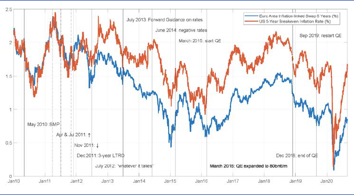
ECB Forum on Central Banking, November 2020
289
between inflation expectations in the US and the euro area emerged in that period
and has persisted since (see Chart 2).
Chart 2
Inflation expectations in the euro area and in the US
Source: Datastream and St Luis Fed Fred database.
These examples suggest that balance sheet policies in the euro area have
potentially large effects on both financial stability and price stability. They also
suggest that these effects are dependent on effective – credible – communication,
and that this communication effectiveness may be undermined when political (and
fiscal) backing for asset purchase programs is called into question. Asset purchases
inevitably have fiscal consequences and, in stressed circumstances, lack of political
support for ECB action can be interpreted by the market as a signal of uncertain
fiscal backing. This uncertainty, as we have seen, impaired the effectiveness of
policy announcements between 2012 and 2014 but it is also the reason why the
Security Market Programme implemented in 2010-2011 had limited effectiveness,
notwithstanding large actual purchases (see Reichlin, 2019 for a discussion on this
point).
For the future, the continuous effectiveness of the new ECB toolbox will depend on
clarification of the principles guiding balance sheet policies in a situation where a
common yield curve of the euro area does not exist and stabilizing financing
conditions implies stabilization of cross-country spreads. In such circumstances it
must be recognized that quasi-fiscal effects of monetary policy operations are
inevitable and therefore a risk management framework must be more clearly
designed. I return to this last point in Section 3.
2.3 The fiscal transmission channels
Another feature of the euro area that has to be considered when analyzing the effect
of monetary policy is how the latter interacts with fiscal policy in the determination of
inflation. Given the decentralized nature of budgetary decisions but also the nature of
ECB Forum on Central Banking, November 2020
290
the fiscal rules, it is not clear whether monetary and fiscal policies have been
coherent or whether cross-winds have prevailed.
Monetary policy – standard or unconventional – has implications for fiscal policy and
fiscal policy has implications for price stability.
The Maastricht Treaty was designed to ensure a rigid separation between monetary
and fiscal policy. The framework corresponds to the idea that monetary policy can
always control the price level, no matter what fiscal authorities do. The consequence
of this idea is the belief that in an asymmetric federation, with a single monetary
policy authority and nineteen fiscal authorities, macroeconomic stability can be
ensured by a combination of a credible and independent central bank targeting price
stability, and fiscal rules setting public deficit and public debt limits. Coordination
between monetary and fiscal policy was deemed not necessary to pin down the price
level and not desirable provided that all authorities followed the rules.
Fiscal-monetary interactions, however, naturally arise via the general government
intertemporal budget constraint. This is true in general and even in a frictionless
model: the price level is determined by both fiscal and monetary action.
At zero interest rate swapping reserves for short term debt is neutral since both
reserves and short-term bonds yield zero interest rate. From the perspective of the
consolidated government – central bank and treasury – QE is just an exchange of
one type of government paper for another. However, as long as QE consists in
buying long-term government bonds, it shortens the maturity of government debt
held in the market other things being equal (i.e. not considering the potential positive
effects on the maturity of newly issued debt).
There are two considerations which are relevant here.
First, monetary policy easing, and especially sovereign bond purchases, reduce the
cost of debt refinancing and frees fiscal space for governments. Governments may
respond by reducing the primary surplus (let’s call this “coordination”) or by
increasing it (let’s call this “cross-winds”). In Antolin-Diaz et al., 2020 we provide
some empirical evidence on the four largest countries of the euro area and show
that, in response to a non-standard monetary easing (decline of the yield curve
slope), primary surpluses have hardly adjusted except for Germany where cross-
winds have prevailed. This is a topic that has to be explored further because
monetary-fiscal policy coordination may be desirable especially at the zero lower
bound and cross-winds could impair the effectiveness of expansionary monetary
policy in relation to price stability.
Second, a key effect of QE is that, by absorbing maturity risk, the central bank is
shifting that risk from the government to its own balance sheet. From the point of
view of the general government the total amount of risk is unchanged but it is
redistributed from Treasury to the central bank. In the euro area these redistributional
effects also have a geographical dimension which depends on the risk sharing
arrangements within the Euro-system.
ECB Forum on Central Banking, November 2020
291
With high levels of public debt, and with large central bank balance sheets, both
potential risks and fiscal-monetary interaction are more visible.
3 Financial stability risks
The policies we are discussing here as well as standard interest rate policy have
implications for the total supply and demand for risk in the economy as well as for
the distribution of this risk amongst the central bank, the banks and the government
balance sheet.
We have discussed fiscal risk in the previous section. Let us now discuss how risk
taking in general may have implications for financial stability.
Take the example of central bank asset purchases and maturity risk. Purchases have
two effects. The first is redistribution of risk: by purchasing long-term assets the
central bank removes maturity risk from banks and other investors and transfers it to
its own balance sheet. The second – which is not assured – is an increase in the
total risk in the economy. This may or may not happen and the outcome essentially
depends on how investors react to the increased incentives to take more leverage or
to invest in riskier assets.
Both supply and demand matter for the amount of risk in the system. If the central
bank buys risky assets and the supply of risk does not adjust, in equilibrium agents
have to hold the same amount of assets as before minus what the central bank has
bought. Intermediaries must become less risky but the total amount of risk in the
economy is unchanged, just redistributed. Only if there is a larger supply of risk in
the system is there an increase in risk in the economy. In other words, the total
amount of risk in the economy changes only if supply responds.
QE aims at increasing the total amount of risk in the economy. It may or may not
succeed and, as we have seen in Section 2, the evidence is mixed. To the extent to
which it succeeds the desirable (for macroeconomic purposes) increase in the
supply of risk may lead to financial instability. Trade-offs between macroeconomic
and financial stability may therefore arise.
This is not the case for “market-making” type of policies. In that case the central
bank intervenes to support financial intermediation by replacing the market in the
intermediation chain and becoming a sort of intermediary of last resort.
Complementarities between macroeconomic and financial stability should dominate
in this case.
Indeed, the experience of the financial crisis shows that complementarities were
strong and stronger than they were thought to be in the first years of the crisis when
the ECB emphasized the so-called “separation principle” between liquidity and
macroeconomic policies. The idea at the time was that the goal of macroeconomic
stability could be achieved by the use of the conventional interest rate instrument
while the goal of financial stability was a separate objective, to be achieved via
innovative liquidity policies.
ECB Forum on Central Banking, November 2020
292
Although financial stability risks may arise as the unintended consequence of
monetary policy aimed at price stability, they can in principle be handled as long as
another policy instrument is available; this is the motivation for the development of
macroprudential tools. This is a truism: multiple objectives can be pursued only with
multiple instruments. In practice, however, we still have to learn how effective
macroprudential policy is and what its fiscal implications are.
4 Managing credit risks
I have made the point that monetary policy – in particular “active” balance sheet
policies – acts by redistributing risks and often fiscal/credit risks. I have also argued
that there is evidence that they are necessary for both monetary and financial
stability although they may also create incentives for “bad” risk taking.
The recent history, however, has also shown that these policies were necessary for
both macro and financial stability and will continue to be so.
With the increasing size of central bank balance sheets and a change in their asset
composition towards risky assets, the issue is how the associated risks can be
managed.
This raises the question of what the right level of capitalization of the euro-system of
central banks is but also what the rules should be for distributing risks among
national central banks. Today, 80% of the assets purchased under the APP and
PEPP programs are risk activities of the national central banks (the potential losses
related to those purchases are not shared among national central banks and neither
are the profits). Moreover, Emergency Liquidity Assistance (ELA) operations are not
subject to the risk sharing rule at all. In principle, a central bank which develops
capital losses must be recapitalized by its own government, but if that government is
itself insolvent, that crisis will inevitably lead either to a bailout or to a fatal crisis for
the single currency.
In principle, a coherent system would be one in which monetary operations involving
risks would be guaranteed by national governments with adequate capital. Capital
contributions and profits and losses would be shared according to the capital key.
Clearly such a system implies a level of risk sharing which is more akin to a fiscal
federation than the one we have now. However, the present arrangements would not
provide a viable solution in case of large losses by a national central bank. If those
losses were caused by the insolvency of the central bank’s home country, there
would be no recapitalization and the national central bank would lose eligibility to be
a counterparty in Target2, with the inevitable consequence of crashing out of the
euro-system. But that crash would imply large losses for those national central banks
which hold claims in Target2 (on this point see Perotti, 2020). Under these
circumstances, a system of full risk sharing, with appropriate rules on capital
adequacy, seems a better alternative. This discussion must be on the table.
ECB Forum on Central Banking, November 2020
293
5 Conclusions
The use of non-standard monetary policy is necessary for financial stability and
macroeconomic objectives. In the monetary union there is an even stronger
motivation due to the vulnerability to liquidity strikes in peripheral countries and the
anti-cyclical dynamics of the spreads of peripheral governments’ bond yields with
respect to the German bund.
As the new instruments developed in the last decade become part of the standard
monetary policy framework, there is a need to develop a framework recognizing that,
while innovative monetary policy is necessary, it may imply credit risk for the central
bank and have distributional effects.
Active balance sheet policies act by redistributing risk from markets to the central
bank and by encouraging an increase in the total supply of risk. While the latter
effect can be addressed – at least in principle – by macroprudential policies, the
former has to be managed by governing the relationship with the fiscal authorities.
The clarity of this relationship is also a key ingredient for the effectiveness of central
bank policies since it is a condition for credibility and of course legitimacy.
To achieve this clarity will require a review of risk sharing arrangements and of the
rules guaranteeing the commitment by governments to provide the necessary capital
to absorb the risks associated with the new policy framework. Any step in this
direction, however, is a step towards some form of fiscal federation and will require a
political process. In the meantime, the single currency remains fragile.
References
Antolin-Diaz, J., Reichlin, L. and Ricco, G. (2020), “Monetary-fiscal cross-winds in
the monetary union”, paper prepared for the 2020 BIS annual conference.
Corsetti, G.C. and Dedola, L. (2016), “The mystery of the printing press: monetary
policy and self-fulfilling debt crises”, Journal of the European Economic Association,
vol. 14, Issue 6,1, pages 1329-1371.
Hasenzagl, T., Pellegrino, F., Reichlin, L. and Ricco, G. (2019), “The inflation puzzle
in the euro area – it’s the trend not the cycle!”, VOX EU, 16 October.
Leombroni M., Vedolin, A., Venter, G. and Whelan, P. (2020), “Central Bank
Communication and the Yield Curve”, Journal of Financial Economics.
Perotti, R. (2020), “Understanding the German criticism of the Target system and the
role of central bank capital”, CEPR discussion paper No. 15067, July.
Reichlin, L. (2019), La Banque Centrale Européenne et la Crise de l’Euro, Fayard
Paris, September.
ECB Forum on Central Banking, November 2020
294
Woodford, M. (2012), “Methods of Policy Accommodation at the Interest-Rate Lower
Bound” in The Changing Policy Landscape, Federal Reserve Bank of Kansas City,
35.

ECB Forum on Central Banking, November 2020
295
Central bank balance sheets and
financial stability
By Hyun Song Shin
1
Abstract
The “dash for cash” during the financial market stress in March 2020 underscores
the importance of elastic nodes in the financial system that can accommodate the
demand for money. Commercial banks are the first line of defence, and central
banks are the second line of defence, both domestically and internationally. The
dash for cash was a dash for dollars primarily, and not all currencies received “dash
for cash” flows. Emerging market currencies depreciated sharply during the stress
episode. Central banks are guardians of the currency, first and foremost. They
should take close note of the exchange rate as a possible guide to future inflation.
1 Elastic nodes and the “dash for cash”
The COVID-19 pandemic delivered a stress test for the financial system when a
large swathe of the non-bank financial intermediary (NBFI) sector came under
significant stress in March 2020 (FSB (2020)). Notable in this episode was the “dash
for cash” where the demand for money or money-like instruments spiked, at the
expense of other assets that do not have the attribute of “moneyness”.
Commercial banks are typically the first line of defence in meeting this higher money
demand, and they do so by granting overdrafts, thereby creating deposits against the
loans granted via the overdraft. Chart 1 is a stylised depiction of this process, where
the commercial bank credits the deposit account of the borrower and simultaneously
books the overdraft amount as a loan. The borrower then acquires money in the form
of commercial bank deposits, but incurs a debt to the bank in the process.
1
Economic Adviser and Head of Research, Bank for International Settlements. I thank Iñaki Aldasoro,
Claudio Borio, Agustín Carstens, Claudio Borio, Paolo Cavallino, Stijn Claessens, Benoît Cœuré,
Benoît Mojon, Aaron Mehrotra, Patrick McGuire, Goetz von Peter, Andreas Schrimpf, Ilhyock Shim, for
helpful comments and discussions. Alberto Americo, Giulio Cornelli, Anamaria Illes, Swapan-Kumar
Pradhan and Jimmy Shek provided excellent research assistance.
ECB Forum on Central Banking, November 2020
296
Chart 1
Commercial bank as elastic node: money creation through overdraft
We can track the increased money holdings through the weekly data on commercial
bank deposits from the Federal Reserve. The left-hand panel of Chart 2 shows the
cumulative increase in deposits at US commercial banks, while the red dots show
the corresponding increase in commercial and industrial (C&I) loans. Indeed, this
pattern is apparent in the immediate aftermath of the bankruptcy of Lehman Brothers
in September 2008.
Chart 2
Flexible nodes in the system can help stem a drying-up of market liquidity
Source: Frost, J. Shin, H.S. and Wierts, P. (2020), “An early stablecoin? The Bank of Amsterdam and the governance of money”, BIS
Working Papers, No 902, November.
Notes: C&I loans = Commercial and industrial loans.
Banks’ money creation role is as old as banks themselves. The right hand panel is
the money creation conducted by the Bank of Amsterdam during the 1763 crisis,
when the Bank purchased silver and gold coins in the open market and credited the
deposit accounts of sellers of these coins, thereby creating money through open
market purchases. This kind of operation is exactly analogous to modern asset
ECB Forum on Central Banking, November 2020
297
purchase programmes of central banks where they purchase safe assets by creating
reserves held by commercial banks. Banks are elastic structures in that their
liabilities can be managed actively by the bank itself in response to a spike in the
demand for money. Stablecoins or money market funds (MMFs) cannot do this. The
difference between a flexible node and a rigid stablecoin is explained further in my
recent paper (see Frost et al. (2020)) on the rise and fall of the Bank of Amsterdam.
2 Elastic nodes in the international context
The role of elastic nodes in meeting the dash for cash was also evident in the
international context in March. The dash for cash raises the question “dash into
which currency?” It turns out that the “dash for cash” was in fact a “dash for dollars”,
and it was the Federal Reserve which played the role of the elastic node in the global
context by supplying dollars through its swap arrangements with other central banks.
Chart 3
Change in cross-border claims of BIS reporting banks and net interoffice assets of
foreign banks in the United States; in billions of US dollars
Notes:
1 Adjusted for break-in-series and exchange fluctuations.
2 Includes central banks and banks unallocated by subsector between intragroup and unrelated banks.
3 Includes non-banks unallocated by subsector.
4 Weekly outstanding amounts since 3 January 2018.
Sources: BIS locational banking statistics (by residence); Federal Reserve H.8 data.
The left-hand panel of Chart 3 shows the change in cross-border claims of BIS-
reporting banks. We see the surge in inter-bank claims in the first quarter of 2020.
The right-hand panel plots the net borrowing by non-US banks operating in the
United States from their headquarters. The flows being channelled into the United
States during the stress period reflects a circular flow of dollars, analogous to the
overdraft diagram above (Chart 1), but with the additional intermediation by the
central bank counterparties in the swap arrangement. The dollars provided under the
central bank swap lines are lent to commercial banks, find their way back to the
United States and end up as reserve balances at the Fed. The circular flow of dollars
is illustrated in the following flow diagram, taken from a recently published BIS
Bulletin (see Aldasoro et al.).
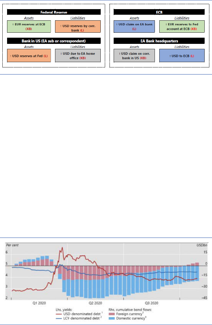
ECB Forum on Central Banking, November 2020
298
Chart 4
Circular flow of dollars resulting from central bank swap lines
The red arrow in Chart 4 is part of the net interoffice liabilities plotted in the right-
hand panel of Chart 3. In this way, cross-border flows can provide a good point of
measurement for broader shifts in global balance sheet adjustments. The fact that it
crosses the border is not economically significant in its own right, but measurement
is often easier at the border – much like the way that a strobe light captures the
snapshot of continuous movements that happen in the dark.
3 Currency dimension and the exchange rate
The dash for cash has a currency dimension. The dash in March was for dollars.
Other currencies fared less well, especially those of emerging market economies.
Chart 5 shows the cumulative flows into and out of emerging market sovereign
bonds, both in domestic currency (in blue bars) and in foreign currency (in pink bars).
Chart 5
Portfolio outflows from EME domestic currency sovereign bond markets have not
reversed
Source: EPFR; JPMorgan Chase; national data; BIS calculations.
Notes:
1 JPMorgan EMBI Global index, stripped spreads.
2 JPMorgan GBI-EM Broad index, yields on traded index.
3 Flows to foreign and blend currency bond funds.
4 Flows to local currency bond funds.
This chart reveals that while spreads have normalised for the domestic currency
sovereign bonds, the flows have not. The outflows from domestic currency sovereign

ECB Forum on Central Banking, November 2020
299
bonds have not been reversed, leaving domestic investors to absorb new issuance,
including by the central bank. In contrast, the dollar-denominated outflows from EME
bonds have now fully reversed. The fact that the flows show such a stark difference
even for the same borrowers suggests that the currency dimension is important.
Even if the debt is issued by the same borrower with the same credit risk profile, the
dash for cash is not into all currencies.
The currency dimension highlights the importance of the exchange rate. During
periods of rapid depreciations of the currency associated with currency crises in
emerging market economies, exchange rate pass-through to inflation tends to be
heightened. Chart 6 shows that pass-through in Latin America was very high during
its years of monetary instability in the 1980s and 1990s. In Asia, pass-through jumps
in 1997, at the time of the Asian Finance Crisis.
In past crises, inflation surged even during periods of depressed economic activity
associated with financial crises. Phillips curve reasoning, which attributes inflation to
overheating of the economy, does not have much bite in such circumstances.
Instead, old-fashioned notions of the value of currency hold sway.
The surge in pass-through need not result in sustained high inflation. However, the
fork in the road is the monetary policy response to fiscal deficits. Past episodes of
monetary instability and high inflation often featured fiscal deficits are financed by the
central bank through money creation.
Perhaps for this reason, forecasts of future inflation outcomes in emerging market
economies using historical data show a role for fiscal deficits in the one year-ahead
inflation outcome density, as shown in Banerjee et al (2020).
Chart 6
Exchange rate changes and future inflation
Correlation coefficient on a 10-year rolling window
Sources: IMF International Financial Statistics; Global Financial Data; national data; authors’ calculations.
Notes: Simple average across individual countries within the panels. Correlation between the changes in the local exchange rate vis-à-
vis the US dollar and the one-quarter forward inflation rate. The level of the exchange rate is positive when the local currency is
deprecating vis-à-vis the US dollar.
Chart 6 shows the one-year ahead forecast inflation density using quantile
regressions where the red density is conditional on a one standard deviation
increase in the fiscal deficit, while other variables are left at their mean levels. We
ECB Forum on Central Banking, November 2020
300
see that the red density is associated with higher levels of inflation, no doubt
reflecting the historical data where higher fiscal deficits were associated with higher
inflation.
The currency is a promise issued by the central bank. To this extent, the central
bank, above all, is the guardian of the currency.
References
Aldasoro, I., Cabanilla, C., Disyatat, P., Ehlers, T., McGuire, P. and von Peter, G.
(2020), “Central bank swap lines and cross-border banking flows”, BIS Bulletin
No 34.
Banerjee, R., Contreras, J., Mehrotra, A. and Zampolli, F. (2020), “Inflation at risk in
advanced and emerging economies”, BIS Working Papers, No 883.
Financial Stability Board (2020), “Holistic review of the March market turmoil”, report
to the G20, 17 November.
Frost, J., Shin, H.S. and Wierts, P. (2020), “An early stablecoin? The Bank of
Amsterdam and the governance of money”, BIS Working Papers, No 902.

© European Central Bank, 2021
Postal address 60640 Frankfurt am Main, Germany
Telephone +49 69 1344 0
Website www.ecb.europa.eu
All rights reserved. Reproduction for educational and non-commercial purposes is permitted provided that the source is acknowledged.
These papers should not be reported as representing the views of the European Central Bank (ECB) or the Eurosystem. The views
expressed are those of the authors and do not necessarily reflect those of the ECB or the Eurosystem.
For specific terminology please refer to the ECB glossary.
PDF ISBN 978-92-899-4728-2, ISSN 2363-3239, doi:10.2866/268938, QB-BN-21-001-EN-N
HTML ISBN 978-92-899-4727-5, ISSN 2363-3239, doi:10.2866/076498, QB-BN-21-001-EN-Q
